Spatial autocorrelation & co

These days I run a fair bit of spatial analysis. And there are three problems that regularly come up:

1. Getting data on compatible geographies
2. Ecological fallacy
3. Spatial autocorrelation

None of these problems is insurmountable, but they are all annoying to various degrees. Often I might ignore them on my first analysis run, but these problems need to be dealt with sooner or later. Which can eat up significant amounts of time. Sometimes the analysis results don’t change much after properly dealing with these issues. Sometimes they change significantly. Sometimes they change dramatically to the extent of reversing the overall interpretation.

There are other issues that come up in analysis too, but these I find regularly in my particular workflows, and these are usually the most time consuming to deal with.

All these problems are fairly well understood, and a lot of ink has already been spilled on each of these. Not all of these problems come up in every setting, but at least one or two of them come up in pretty much any research dealing with spatial data. And despite these problems being well-known, I am surprised how many papers don’t adequately deal with them, or even completely ignore them.

For the first problem we have written the tongfen package, that focuses on Canadian census data and greatly simplifies the common task of making census data comparable through time, and also allows to estimate data on unrelated custom geographies.

The ecological fallacy comes into play when trying to extract information on individual level behaviour from ecological level correlations. This comes up when individual level cross-tabs aren’t available, for example when mixing data from different sources. There are a number of approaches to deal with this, in particular Gary King’s elegant methods. Dealing with this generally requires a lot of hand-holding, we have not found implementations that are easy to use and automate the error detection and iterations that we found are usually required. We will leave this for a separate future blog post.

This leaves us with the last issue on our list, spatial autocorrelation, and I want to take this opportunity to walk through a detailed example myself, complete with code for reproducibility.

Spatial autocorrelation

When fitting models, we need to check if the assumptions of the model are satisfied. When working with spatial data, we impose an additional assumption on most models. That the residuals aren’t spatially autocorrelated.

Spatial autocorrelation boils down to the fact that nearby things tend to be more related than far away things. When residuals of a fitted model exhibit spatial autocorrelation the model is facing two problems. The individual observations that fed the model can’t be treated as statistically independent. This can inflate p-values in linear models, and bias model validation done via standard random train/test data split. Moreover, it can introduce sizable (and statistically highly significant) spurious correlations.

And the most annoying part is that when building models from real life spatial processes, autocorrelation in residuals tends to be the norm rather than the exception.

To better understand why I obsess so much about this these days, let’s consider an example. This is reproducing part of an excellent post by Morgan Kelly where he explores the likelihood that improperly handled spatial autocorrelation invalidates results of selected published economics research.

Following Morgan Kelly, we take a 100 by 100 square, and assign values to each cell via two independent random spatial processes. The word spatial here means that the process behaves like spatial processes we see in nature. Say a temperature distribution. Or soil contamination. Or how demographic variables like median income, tenure or mode of transportation to work tend to distribute. That is, a random process with spatial autocorrelation.

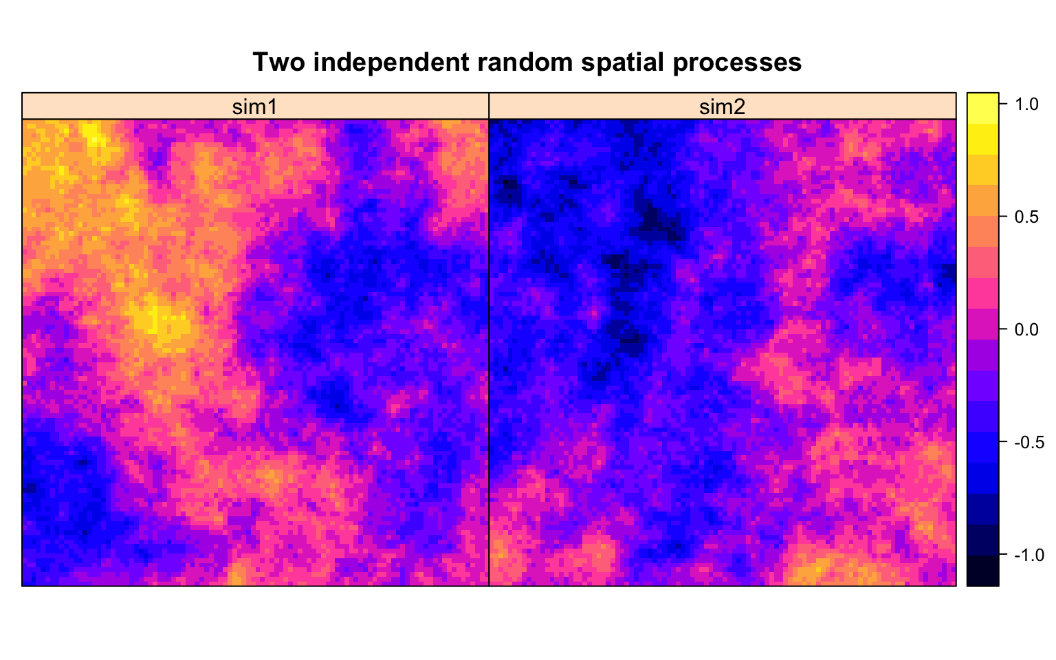
These pictures show the values of our two random spatial processes, which we called sim1 and sim2. They are modelled as a constant model with spatial noise, we refer those interested in details to the code. We think of sim1 and sim2 taking values over the same square.

Next we will sample the square at 80 randomly chosen points, with locations shown in white below, and correlate the values of sim1 at these points to those of sim2 at these points.

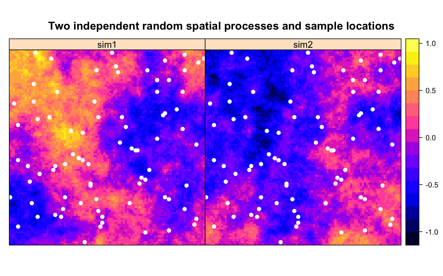
One can think of this as correlating e.g. air contamination with density of factories. Or income with home values. Except using two independent random spatial processes instead of real data. Since the two processes sim1 and sim2 are independent random processes, we would expect their values at our sample points to be uncorrelated.

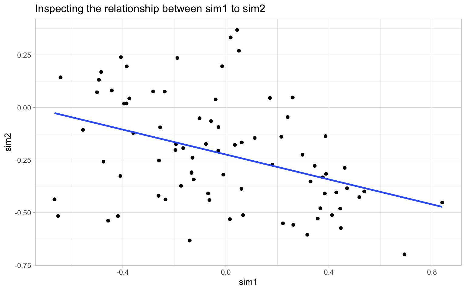
Visual inspection shows this not to be true. More precisely we get a strong and highly significant correlation between these variables, with low but significant adjusted \(R^2\) of 0.15.

	Estimate	Std. Error	t value	Pr(>|t|)
(Intercept)	-0.13	0.05	-2.82	6e-03
sim2	-0.53	0.14	-3.82	3e-04

We can proceed with standard checks to see how the residuals are distributed.

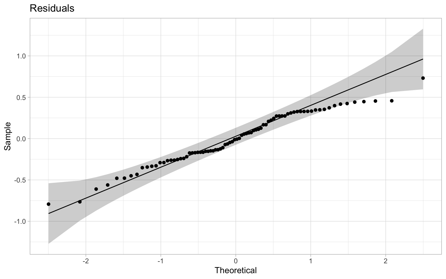
Things looks reasonably normal on this front. To understand what goes wrong here we plot the associated variogram.

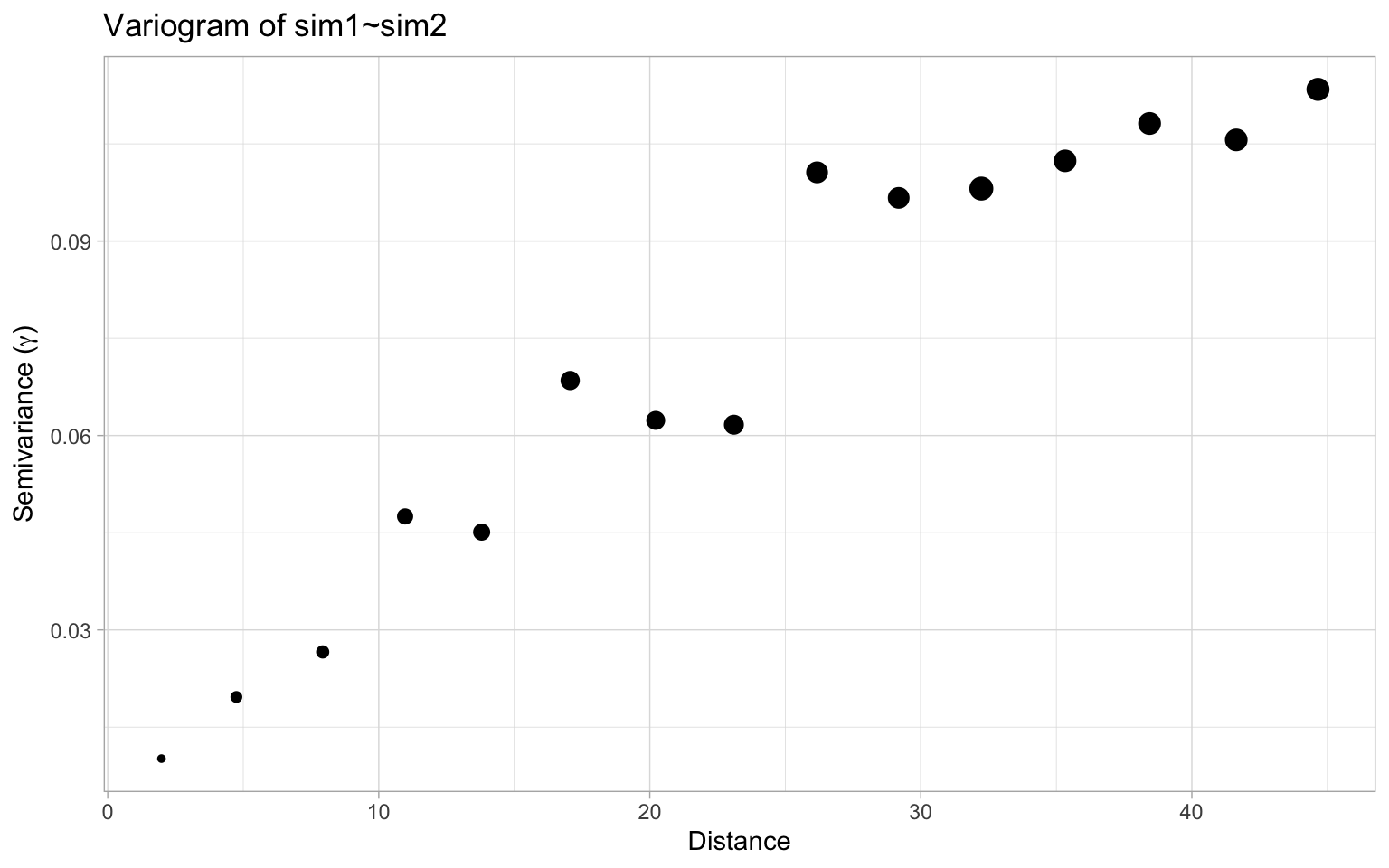
This shows high autocorrelation at least up to a distance of about 25. Guided by this we can produce neighbour weights up to a distance of 25 scaled by inverse distance and check Moran’s I statistic, which clocks in with a statistic of 0.71 and a p-value at or below 1e-04, the resolution of our Monte Carlo simulation of 10,000 runs.

As expected, the model residuals are highly autocorrelated. Had we not checked this, we might have concluded that sim1 and sim2 are highly correlated, when in fact the correlation is entirely due to spatial autocorrelation.

Of course this is not news to researchers and has been well documented before, which is why I am so surprised to keep coming across research papers in economics, planning, or geography that does not even check from spatial autocorrelation. Morgan Kelly runs through a couple of such examples in his post.

How to deal with spatial autocorrelation

Just because regression residuals exhibit significant autocorrelation does not mean that the analysis is doomed. There are ways to deal with this problem. Probably the best way is to identify a non-random spatial process that can explain the autocorrelation. For example, if you are fitting a model to housing prices and you see strong spatial autocorrelation in residuals, you may be missing some important neighbourhood-level features. Maybe school catchment areas, or patterns in street trees, areas with ground slope that favours views vs areas that don’t have views, or proximity to amenities. Plotting the residuals can help reveal these patterns. If this approach is successful it’s a double win. It reduces autocorrelation and strengthens the model by adding missing variables with explanatory power.

But often this strategy does not work. And if it does it usually only reduces autocorrelation, but does not remove it to the extent that it can be ignored.

Aggregating data based on the range of the autocorrelation will reduce the autocorrelation, but it also reduces the data we want to use to build our model from. Generally a better strategy is to select a model that explicitly deals with autocorrelation. Typical choices are spatial lag or spatial error models. These are linear models that add a spatially lagged term to a linear regression model. The spatialreg package in R implements several choices, but they only work for regular linear models, possibly with weights. For more complex models, even just lasso or ridge regression, one needs to custom build this by hand. Having more flexible ready-made processes for building such models would be helpful and might help increase adoption.

For our case at hand, we choose a spatial error model of the form, \[ y = X \beta + u, \hspace{1cm} u = \lambda W u + \epsilon \] where \(w\) is the spatial weights term. The model picks up \(\lambda\) of 0.68 and an overall superior (AIC) fit compared to our previous naive linear model with pseudo \(R^2\) of 0.58. The coefficients however aren’t statistically different from zero.

	Estimate	Std. Error	z value	Pr(>|z|)
(Intercept)	-0.03	0.07	-0.4	0.69
sim2	-0.03	0.13	-0.2	0.84

In summary, the spatial error model successfully picks out the spatial autocorrelation and finds no evidence for correlation between our two random spatial processes sim1 and sim2. Checking Moran’s I we have a statistic of 0.0092 and a p-value of 0.43, providing no evidence of remaining spatial autocorrelation.

Checking in on the residuals we notice a slight increase in performance too, with residuals better fitting the normality assumption.

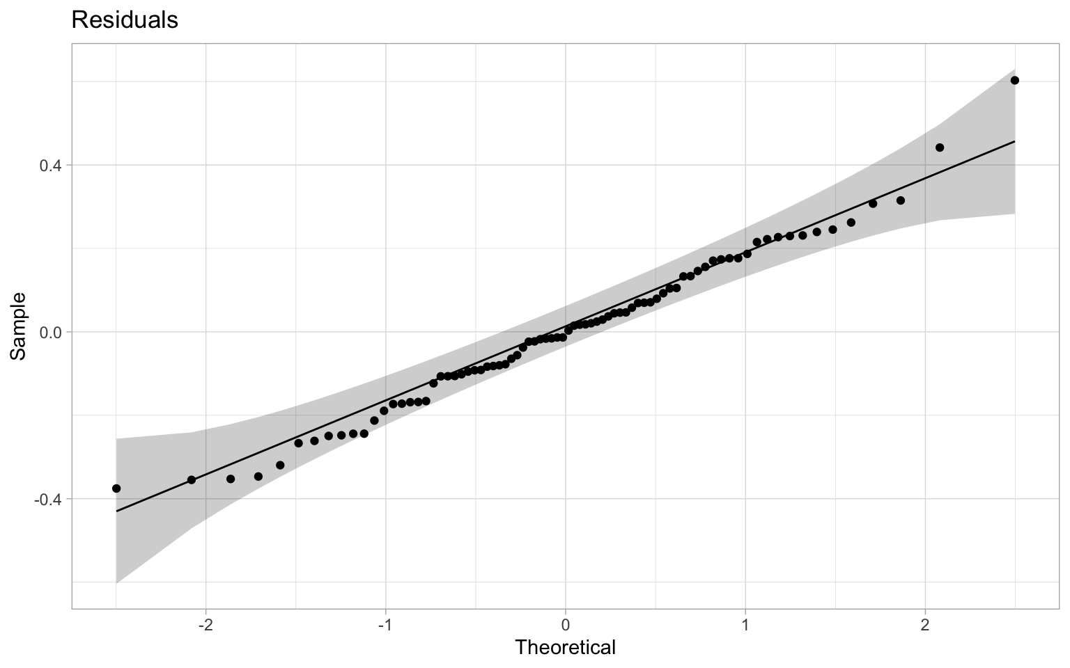
Our spatial error model was fully successful in picking up the spatial autocorrelation and removing the spurious correlation. This is the best-case scenario, in real life things usually aren’t that clean.

The nitty-gritty

Things don’t always go this smoothly as in this toy example. In practice, things tend to get more messy and it can be at times challenging to properly identify the correct patterns of spatial autocorrelation and properly deal with them.

It should be said that spatial autocorrelation does not always negatively affect naive regression results. It’s the nature of random processes that they can sometimes produce positive spurious correlation, sometimes negative spurious correlations, and sometimes no significant correlation.

To exemplify this, we can re-run our initial random spatial processes for sim1 and sim2 a number of times and compare the results of running a naive regression.

Run	Estimate	Std. Error	t value	Pr(>|t|)	r squared
1	-0.53	0.14	-3.82	0.00027	0.15
2	0.30	0.08	3.89	0.00021	0.15
3	0.08	0.12	0.62	0.53756	-0.01
4	0.01	0.07	0.16	0.87241	-0.01
5	0.10	0.10	1.00	0.32031	0.00
6	0.35	0.09	3.73	0.00036	0.14
7	-0.18	0.08	-2.15	0.03462	0.04
8	0.07	0.11	0.64	0.52476	-0.01
9	0.25	0.14	1.72	0.08867	0.02
10	0.14	0.09	1.57	0.11995	0.02
11	-0.54	0.13	-4.01	0.00014	0.16
12	-0.55	0.12	-4.70	0.00001	0.21
13	0.58	0.11	5.03	0.00000	0.24
14	0.23	0.11	2.11	0.03791	0.04
15	0.34	0.13	2.55	0.01259	0.07
16	-0.02	0.17	-0.09	0.93039	-0.01
17	0.07	0.09	0.75	0.45801	-0.01
18	0.00	0.14	-0.03	0.97316	-0.01
19	0.05	0.08	0.60	0.55069	-0.01
20	-0.25	0.06	-4.25	0.00006	0.18

We see that 10 of our 20 runs give statistically significant correlations at at least the 0.05 level. In that sense, our initial example was somewhat engineered in that we chose processes that did yield significant autocorrelation of the residuals. But we did not have to try very hard to get one of these.

The spatial process we used to generate the data used an exponential variogram model with range of 25, which our diagnostic variogram we plotted above correctly identified. Changing the range will change the frequency with which random processes will produce statistically significant spurious correlations. But even in cases where spatial autocorrelation does not negatively impact model coefficients, accounting for spatial autocorrelation will still increase overall model performance.

Validation splits

A related issue with spatial data comes up when splitting data into test and training data. Typically one just splits the dataset randomly, but this is problematic when dealing with spatial data. The idea behind splitting data is that the two subsets are uncorrelated, so if one is used for model training the other can give an unbiased measure of model performance. But in the presence of spatial autocorrelation, a random split into training and test data will not result in uncorrelated subsets. In particular, if we select a random split in our above example, the test data will confirm the spurious correlation we find using the training data.

To better show this we generate 500 random points to evaluate our original model at, and we take an 80:20 split into training and test data. We then evaluate a naive linear model trained on the training data on both the training and test data and compare the results.

Metric	Train	Test
rmse	0.29	0.30
rsq	0.26	0.28
mae	0.24	0.24

The testing data does not pick up on the spurious correlation. The problem is that our testing and training data are correlated via spatial autocorrelation. To pick up statistically independent test data we can’t rely on simple random sampling but should pick up random blocks of data based on the range of the autocorrelation. There are several R packages available for data splitting adapted to spatial data, for example the mlr package. To understand the difference we visualize the splits of the data using spatial and non-spatial splitting methods.

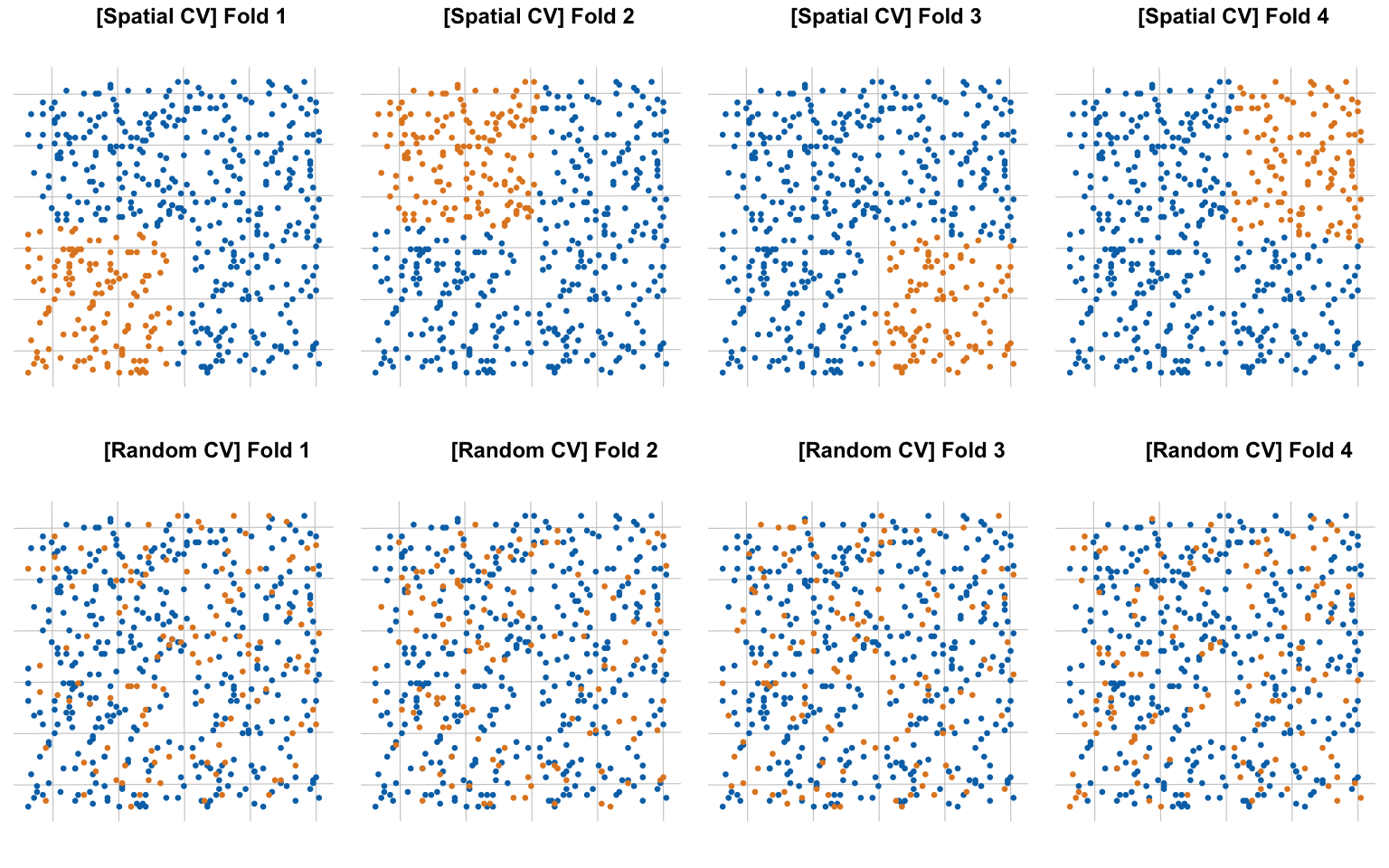
Using 4-fold spatial partitioning we can look at the performance of linear models trained on our training data by evaluating it on the test data on each fold.

Metric	Fold 1	Fold 2	Fold 3	Fold 4
rmse	0.25	0.27	0.41	0.42
rsq	0.24	-0.25	-0.80	-1.54
mae	0.19	0.22	0.35	0.37
slope	-0.58	-0.72	-0.68	-0.26

We notice significantly higher errors and lower (pseudo) \(R^2\) in all but one of the runs. There is a sizable variation in the correlation slope across the runs. When using spatial partitioning of train and test data, the spatial autocorrelation manifests itself in form of increased discrepancy between train and test data, and gives a more accurate picture of overall model performance. In our case, the pseudo \(R^2\) tells us that the models generated from the test data are non-informative at best.

Upshot

It is difficult to evaluate the validity of analysis based on spatial data without checking for spatial autocorrelation, and properly dealing with it if necessary. Despite this, I keep coming across studies in economics, planning, geography and other social sciences that don’t check for spatial autocorrelation despite relying heavily on spatial data.

These disciplines started out doing spatial analysis at times when awareness and understanding of spatial autocorrelation was low, so it is understandable when older research has ignored this issue. But I frequently come across this in recent research too. I suspect this is a case of collective complacency.

The change to include spatial autocorrelation as a necessary check for any published work is bound to happen eventually. This is also sure to trigger a replication effort that checks how results in key papers hold up when spatial autocorrelation is accounted for.

As usual, the code for this post is available on GitHub in case people want to further investigate spatial autocorrelation.