At this stage in the pandemic there is good news and bad news. The good news is that vaccines are ramping up. And change in dosing schedule means more people are getting some level of protection earlier. The bad news is that variants of concern, or VOCs, are on the rise in BC. We have a decent intuition how each one of these changes our pandemic, but unclear how they interact. Thus, it’s time for some modelling. We will keep the model as simple as possible, yet complex enough to capture the interaction between VOCs and vaccinations.
Before we can do modelling we have to assemble the main ingredients.
Vaccinations
We need to understand how many vaccine doses we are getting at what point in time. The three vaccines we are getting in BC are about equally effective, we will assume a 90% efficacy in blocking transmissions starting two weeks after getting the first dose. We still don’t have good data on the transmission blocking ability of vaccinations, but early reports are encouraging and we go with the optimistic estimate for this post. And we will assume that we are fairly efficient in getting the vaccines into people’s arms, on average within one week of delivery.
PHAC has a rough vaccination delivery schedule that we can scrape.
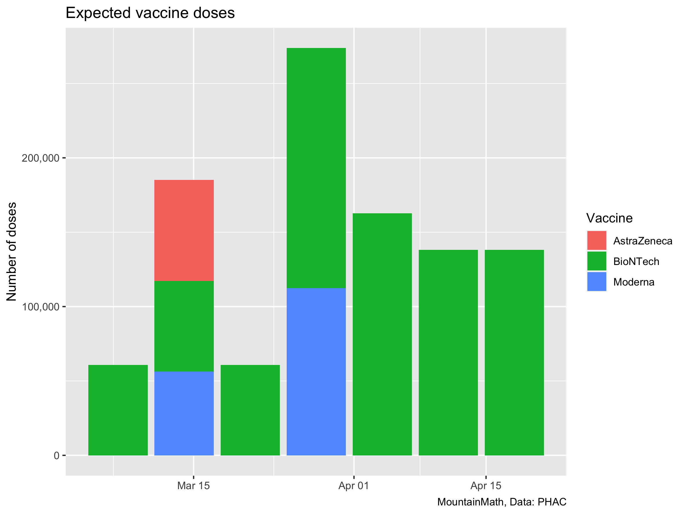 We are interested in the vaccine we are getting now, so we start counting the patch of BioNTech vaccines we got in March. Cumulatively that’s about 1 million doses.
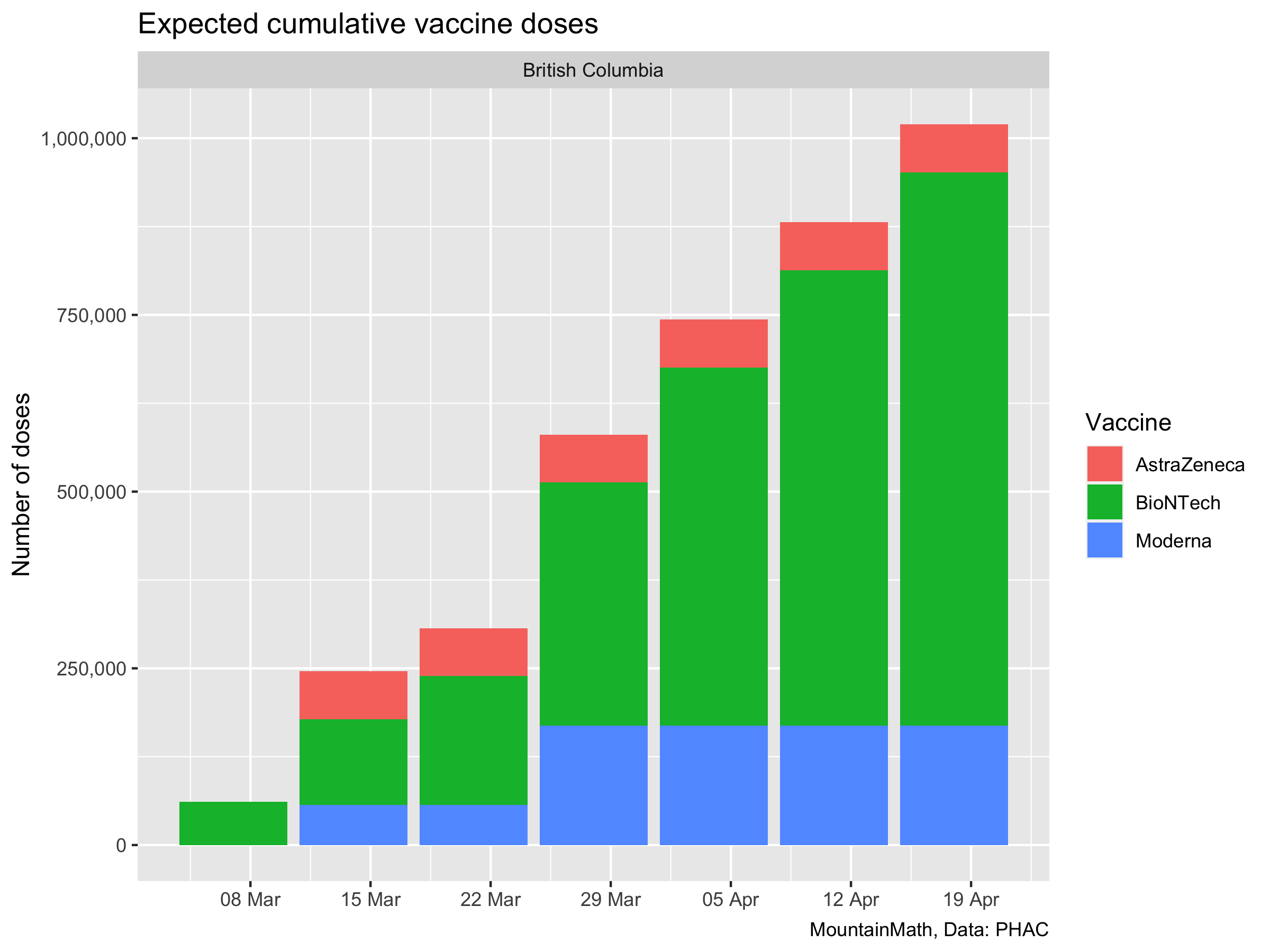
That gives us the data we need to estimate roughly how many people we will vaccinate and how much immunity this will yield. In our simple model we will not distinguish people for whom the vaccine did not grant immunity from people that have not gotten the vaccine. It’s not that hard to do, but it does not make a difference to the model since we aren’t looking at outcomes like hospitalizations and deaths where partial immunity still matters. And we aren’t modelling long enough timeframes where it would matter that we can’t pinpoint ahead of time from whom the vaccines will be less effective.
Variants of concern
Here the problem starts: unlike Ontario, BC still does not release useful data on variants of concern. That means that the share of cases that are variants of concern right now can only be guessed at. Just last week our PHO said that she believes variants of concern hover around 1%, which we find highly questionable. That may have been the state of things in early February, from the data we do see, we believe a better guess would be about 10% at this point in time. But it may well be only 5% or already 15%. The continued refusal to release daily N501Y screening results to allow painting a decent picture of VOC development in BC is frustrating.
The other part we need to understand is the growth rate advantage that variants of concern have. Studies based on UK data have pegged B.1.1.7, the main variant in circulation in BC, to be about 1.5 times more infectious than regular COVID-19. That was based on PCR SGTF as a proxy for B.1.1.7. It’s a pretty decent proxy. Although there is some noise that probably should be dealt with when estimating the growth rate advantage. (Dean Karlen has a cool approach to deal with this, which got me interested in running these kind of estimates.)
Denmark does a lot of whole genome sequencing and is probably the cleanest data to look at the B.1.1.7 growth rate advantage. To estimate the growth rate advantage we note that over short time periods where behaviour and the susceptible population is relatively constant, the number of cases \(C_0(t)\) and \(C_v(t)\) for regular and variant cases is well approximated by \[ C_0(t) = C_0 e^{r_0t}, \qquad C_v(t) = C_v e^{(r_a+r_0)t}, \] where \(C_0\) and \(C_v\) are the number of regular and variant COVID-19 cases at time 0, \(r_0\) is the base growth rate for regular COVID-19 and \(r_a\) is the growth rate advantage of the B.1.1.7 variant. Taking the ratio of variant to non-variant cases
\[ \kappa = \frac{C_v(t)}{C_0(t)} = \frac{C_v}{C_0} e^{r_at}, \qquad\qquad \log(\kappa) = \hat c + r_a\cdot t \] we see that the growth rate advantage is simply the slope of the log of the ratios over time. That’s easy to estimate from the data.
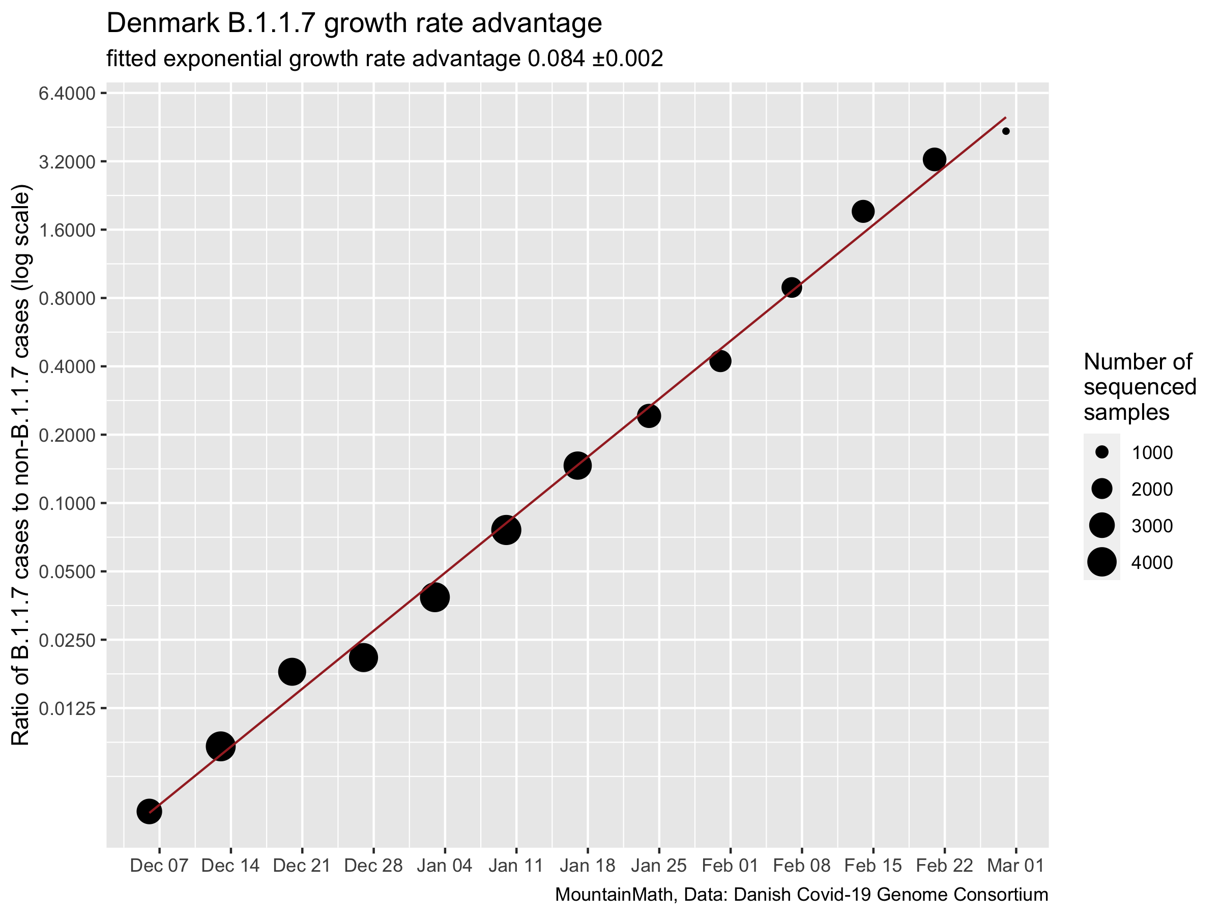
The fit is really tight, in Denmark B.1.1.7 has been consistently growing at a rate of 0.084 ±0.002 faster than regular COVID-19. Will the same be true in BC? We don’t know for sure, but we can look at the N501Y proxy data from Ontario for some clues on how B.1.1.7 behaves in Canada. N501Y is not the same as B.1.1.7, but should still be a cleaner proxy than SGTF. Let’s take a look.
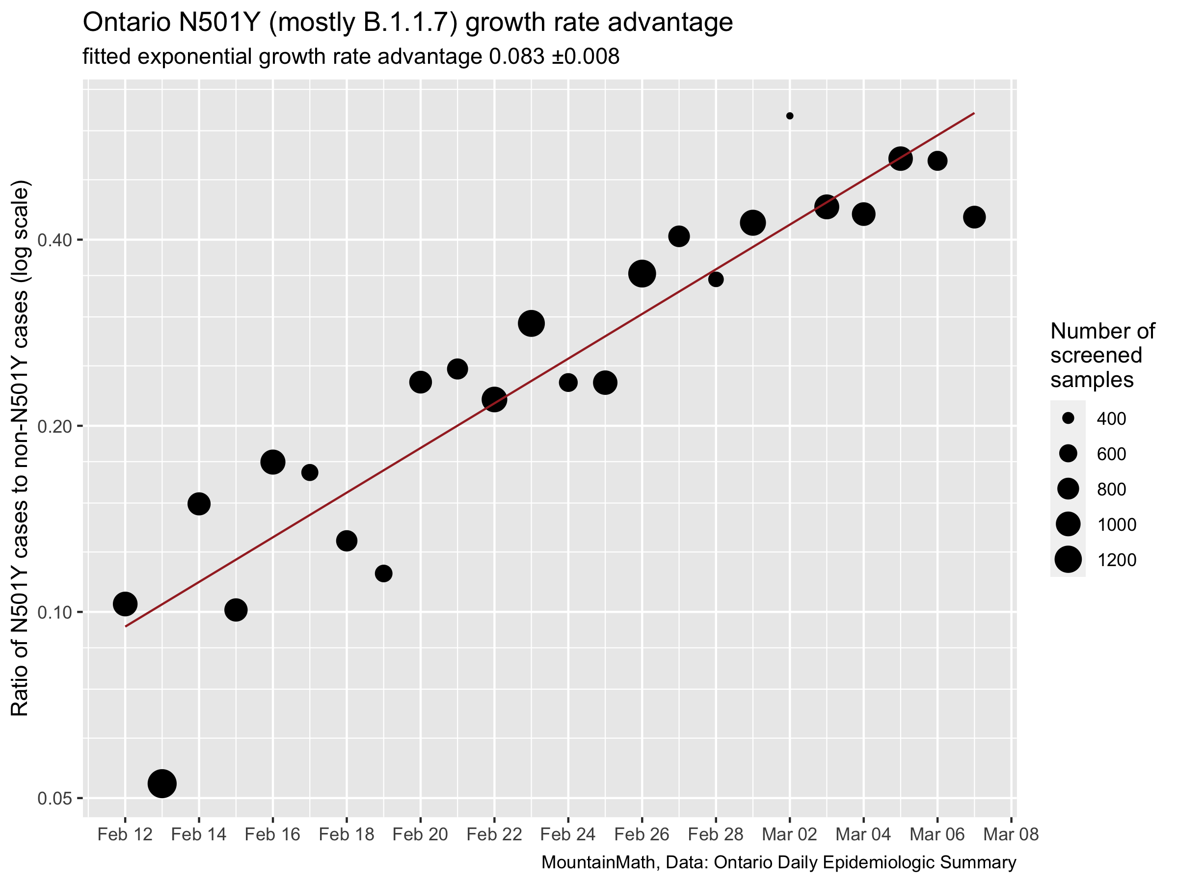
It’s definitely more messy, Ontario does less screening than Denmark does whole genome sequencing. But the overall relationship comes out remarkably similar. We will be assuming a transmission advantage of 0.084 for this post. (There are some technical details here that we are glossing over, but they are minor.)
For this post we are not interested in the question of more severe outcomes of variants of concern since we only look at case counts. Moreover, we will ignore the question of immune escape of variants because we don’t have good data on this. But these are serious concerns that more rigorous modelling needs to include.
SIR Model with Vaccination
For this we have to put in slightly more work than in previous posts where we ran a simple exponential model to account for vaccination. Instead of typing out the equations we just show the code for the standard SIR model that we have extended to include vaccinations and also keep track of cumulative infections from which we can recover daily case counts.
model.vaxx <- function(times,yinit,vaccination_rate,paramters){
  SIR_model <- function(time,yinit,paramters){
    with(as.list(c(yinit,paramters)), {
      vr <- vaccination_rate(time)

      dSusceptible <- -beta*Infected*Susceptible - vr
      dCumulativeInfected  <- beta*Infected*Susceptible
      dInfected  <- beta*Infected*Susceptible - gamma*Infected
      dRecovered <- gamma*Infected
      dVaccinated <- vr

      return(list(c(dSusceptible, dInfected, dCumulativeInfected, dRecovered,dVaccinated)))})
  }

ode(func = SIR_model,times = times,y = yinit,parms = paramters) %>%
      as_tibble() %>%
      mutate_all(as.numeric)
}
Keen eyes will notice that we did not set up separate compartments for variant and regular COVID-19. Instead we will run this as two separate simulations, the difference is that in this setup we allow people in theory to be infected by both, regular COVID-19 and a variant. But that’s going to be very rare and won’t affect the outcomes much as most immunity comes from vaccinations and not from infections. We feel that keeping the model simple is worth the tradeoff. (And we are lazy.)
To start let’s look at the effect of our ramped-up vaccination schedule compared to continuing vaccinating only about 2% of the population per month as we have been doing up to now. For now, let’s forget about variants and pretend they did not exist.
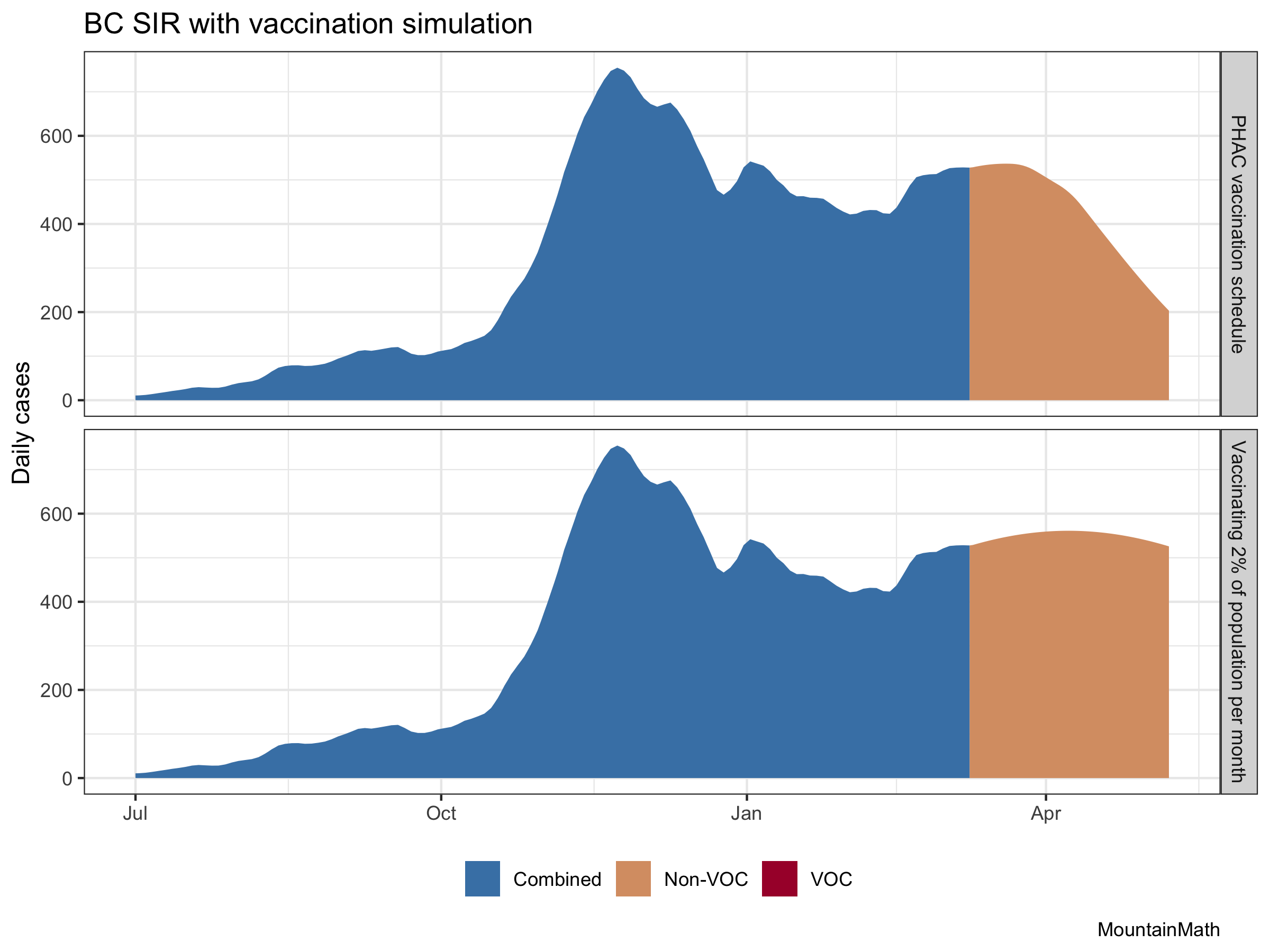
The vaccination effect is clearly visible. There are several assumptions baked into this. One is our initial growth rate, which we set to a very mild increase in cases. The other is how we vaccinate. We know that our age-based vaccination schedule won’t be as good at reducing transmissions as other ways to vaccinate, including vaccinating randomly. This means that the effect of the vaccinations on cases won’t be quite as pronounced as in the above graph. But it will still be strong.
Let’s see what happens when we add VOC into the mix. Especially for B.1.1.7 we got really good data on the transmissibility advantage as outlined above. In BC we don’t really know what share of current cases are variants, but 10% is probably a decent guess.
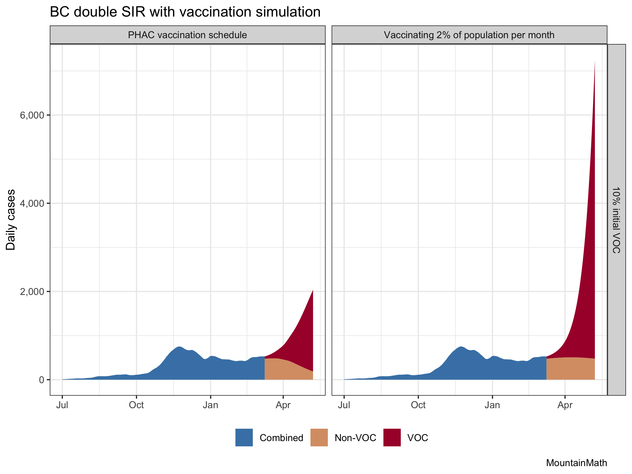
That gives an idea of how bad that added transmissibility really is, and how much the accelerated vaccine schedule is helping. (Although this is likely over-estimating the vaccine effect a bit.) And it also shows that even with the current vaccine schedule, variants of concern are very … concerning. Let’s focus in on our vaccination schedule to get a better image.
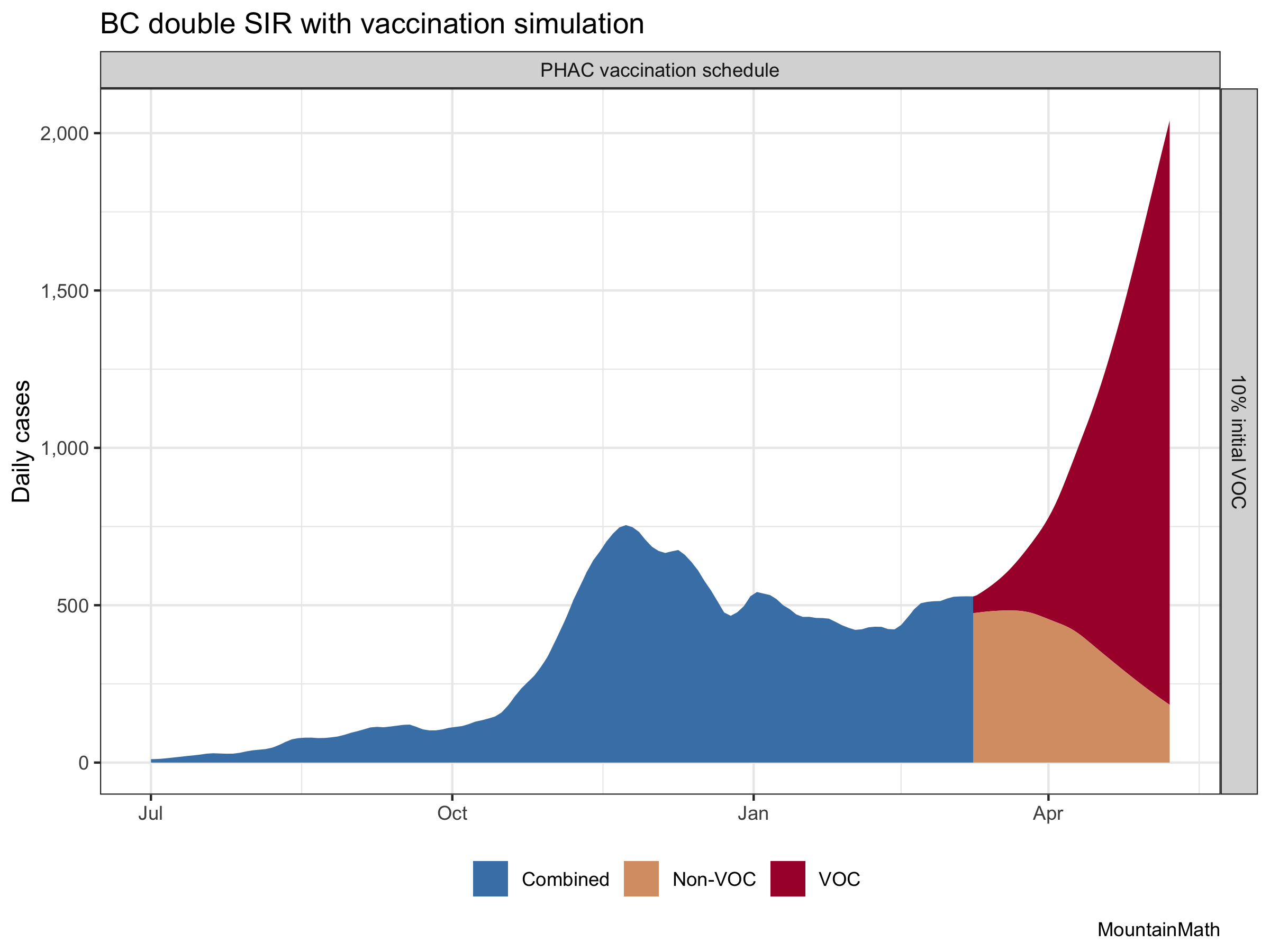
Focusing vaccinations on older populations helps keep mortality low in face of higher case counts. But this does not address problems like Long COVID-19. And additionally, we have now good evidence that B.1.1.7 has higher morbidity and mortality than regular COVID-19, which may well outweigh the reduction in mortality achieved through our vaccines. (Someone should model that!)
But what about the assumption that we currently have 10% variants of concern? Since BC does not release timely counts with dates and denominators, we are adding graphs for 5% or 15%
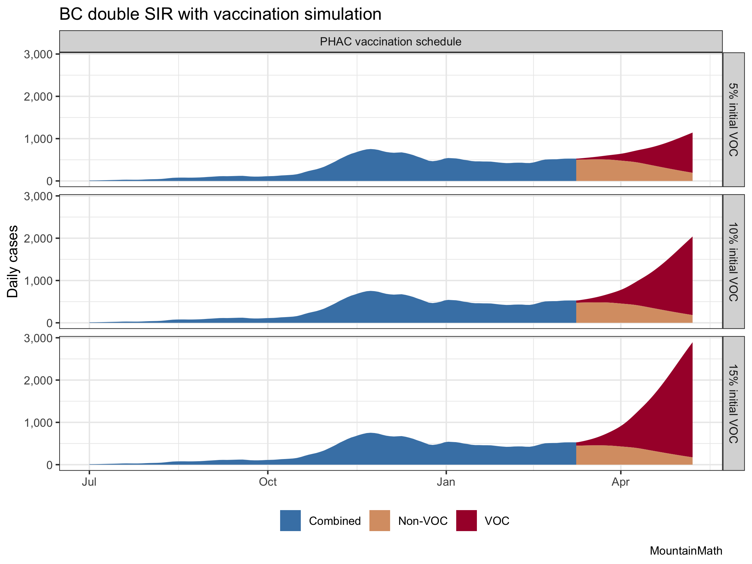
The change in the VOC portion is large, the change in non-VOC cases is largely irrelevant. It shows how important it is to get a decent read on how many variant cases we have right now. That range of assumptions is too large to robustly base policy on.
This is a good time to remind readers that these are projections, and they show what will likely happen if there are no changes in regulations or behaviour. If we open up more, cases will likely rise faster. If we add restrictions, case growth will slow down.
Some people have expressed hopes that warmer weather will bring down case counts. Unfortunately there is little evidence that this will happen to an appreciable degree. And our experience last fall has shown that case growth was quite uniform between July and early November, with the exception of a short period of lower growth around September.
As usual, the code is available on GitHub for anyone to reproduce or adapt for their own purposes.
Reproducibility receipt
## [1] "2021-03-12 10:08:11 PST"## Local: master /Users/jens/Google Drive/R/mountaindoodles
## Remote: master @ origin (https://github.com/mountainMath/doodles.git)
## Head: [363726f] 2021-03-11: vaxx-vs-vocs## R version 4.0.3 (2020-10-10)
## Platform: x86_64-apple-darwin17.0 (64-bit)
## Running under: macOS Big Sur 10.16
##
## Matrix products: default
## BLAS: /Library/Frameworks/R.framework/Versions/4.0/Resources/lib/libRblas.dylib
## LAPACK: /Library/Frameworks/R.framework/Versions/4.0/Resources/lib/libRlapack.dylib
##
## locale:
## [1] en_CA.UTF-8/en_CA.UTF-8/en_CA.UTF-8/C/en_CA.UTF-8/en_CA.UTF-8
##
## attached base packages:
## [1] stats graphics grDevices utils datasets methods base
##
## other attached packages:
## [1] mountainmathHelpers_0.1.2 broom_0.7.4
## [3] deSolve_1.28 forcats_0.5.0
## [5] stringr_1.4.0 dplyr_1.0.4
## [7] purrr_0.3.4 readr_1.4.0
## [9] tidyr_1.1.3 tibble_3.0.4
## [11] ggplot2_3.3.3 tidyverse_1.3.0
##
## loaded via a namespace (and not attached):
## [1] tidyselect_1.1.0 xfun_0.18 haven_2.3.1 colorspace_2.0-0
## [5] vctrs_0.3.6 generics_0.1.0 htmltools_0.5.0 yaml_2.2.1
## [9] blob_1.2.1 rlang_0.4.9 pillar_1.4.7 glue_1.4.2
## [13] withr_2.3.0 DBI_1.1.0 dbplyr_1.4.4 modelr_0.1.8
## [17] readxl_1.3.1 lifecycle_0.2.0 munsell_0.5.0 blogdown_0.19
## [21] gtable_0.3.0 cellranger_1.1.0 rvest_0.3.6 evaluate_0.14
## [25] knitr_1.30 fansi_0.4.1 Rcpp_1.0.5 scales_1.1.1
## [29] backports_1.2.0 jsonlite_1.7.2 fs_1.4.1 hms_0.5.3
## [33] digest_0.6.27 stringi_1.5.3 bookdown_0.19 grid_4.0.3
## [37] cli_2.2.0 tools_4.0.3 magrittr_2.0.1 crayon_1.3.4
## [41] pkgconfig_2.0.3 ellipsis_0.3.1 xml2_1.3.2 reprex_0.3.0
## [45] lubridate_1.7.9.2 assertthat_0.2.1 rmarkdown_2.7 httr_1.4.2
## [49] rstudioapi_0.13 R6_2.5.0 git2r_0.27.1 compiler_4.0.3Reuse
Citation
@misc{vaxx-vs-vocs.2021,
  author = {{von Bergmann}, Jens},
  title = {Vaxx Vs {VOCs}},
  date = {2021-03-10},
  url = {https://doodles.mountainmath.ca/posts/2021-03-10-vaxx-vs-vocs/},
  langid = {en}
}
