(Joint with Nathan Lauster and cross-posted at HomeFreeSociology)
We’re getting better and more accessible datasets for exploring land use change all the time. We have played with the Global Human Settlement Layer (GHSL) data in the past, where we looked at the population data on a 250m grid to compare how different city’s population distribute spatially, as well as the 1975, 1990, 2000, 2015 time series to see how it changed over time. These GHSL population datasets take a variety of input data to build, one part is census or other population-based datasets, the other is the built-out area derived from satellite data that is used to estimate population data at the fine 250m grid.
The emergence of fairly high quality global datasets is quite remarkable, and the ability to go back in time by having these estimates at several points in time back to the mid-70s is amazing.
The city density post was just a first excursion into this data, there is a lot more than can be learned from it. The next logical step - inspired in part by a recent Washington Post piece - is to more closely examine the built-out area timelines that went into making the global population density dataset, and give that data a light workout to better assess it’s strengths and limitations. The dataset comes at an extremely fine 30m resolution, where the extent of the built-out area was estimated off of Landsat satellite data at 1975, 1990, 2000, and 2014.
So let’s do it! To get started we take a look at the built-out area of Canadian metropolitan areas. Here we look at a circular area around the centres of the regions, 40km radius for the larger areas and 25km for the smaller ones, and colour them depending of by when they were built out.
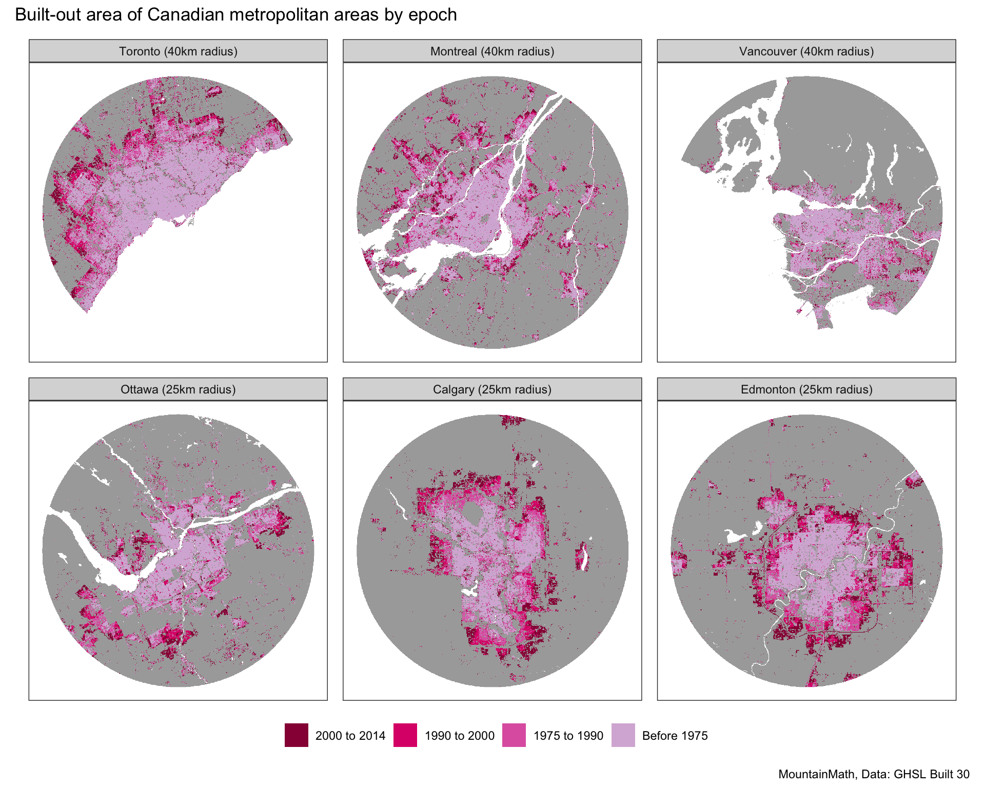 All cities have a light pink centre and have been sprawling outward, but at quite different rates. More recent build-out seems scant in Vancouver, but quite prominent in Calgary and Edmonton. We can directly quantify how much of the current built-up area has been built out across each of the epochs.
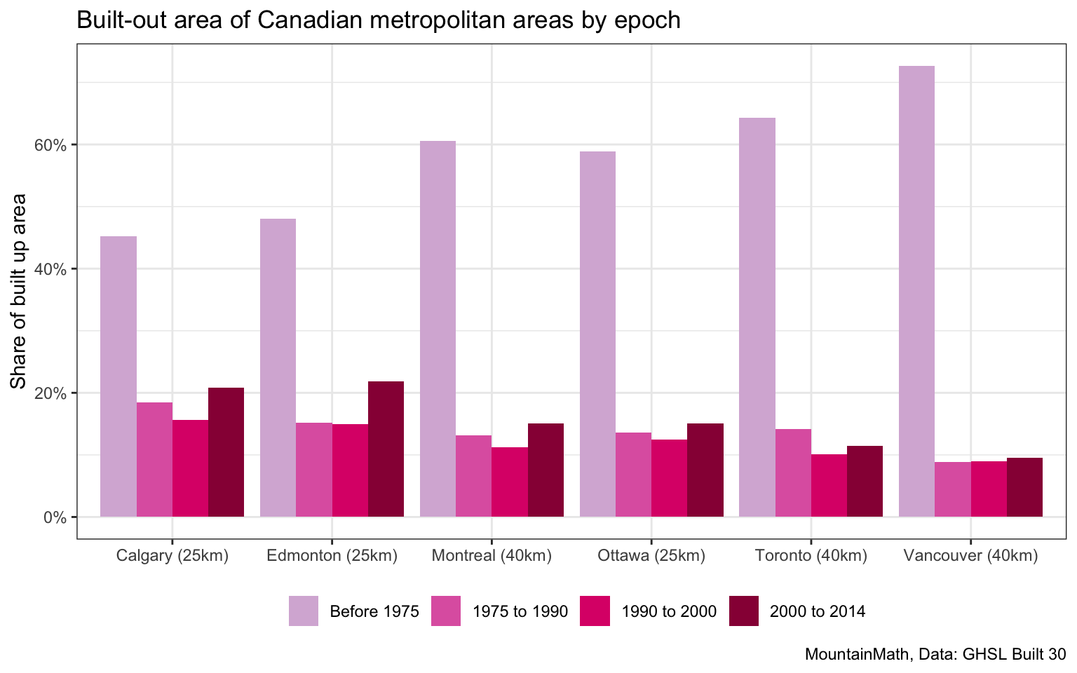
Here we get confirmation that Vancouver has remained the most contained since 1975 (right around the time BC put the Agricultural Land Reserve into place), followed by Toronto (with its more recently established Green Belt). By contrast, Calgary and Edmonton have sprawled outward, more than doubling their built footprint since 1975.
An additional glory of the data is its international coverage.
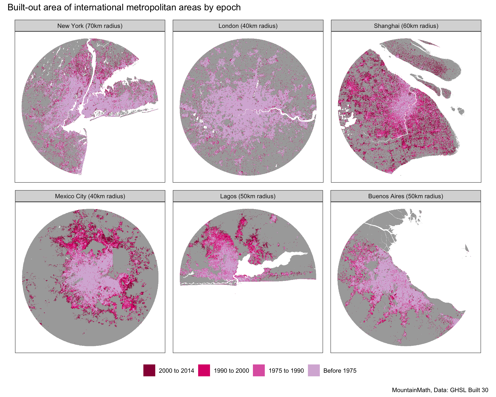
We can pull data from just about anywhere! Here get a glimpse of how old Metropoles of the 19th and 20th Centuries, like London and New York, compare to some of the faster growing megacities in the 21st Century.
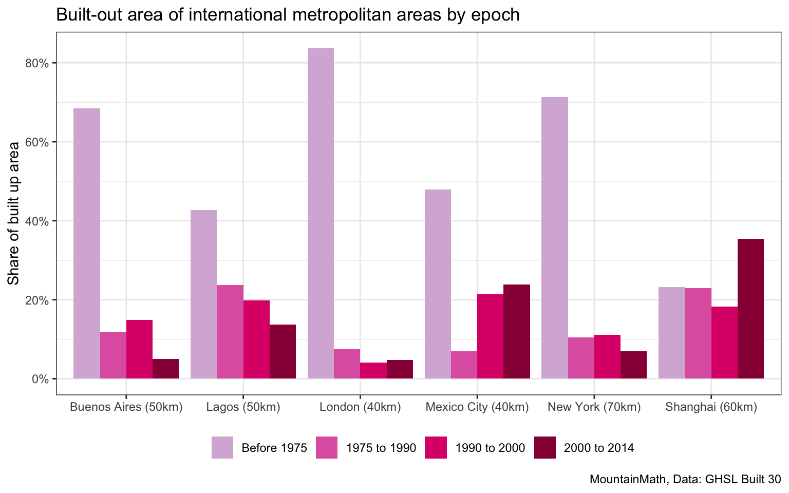
More of Shanghai appears to have been built out between 2000 and 2015 than existed in 1975!
Mystery city came
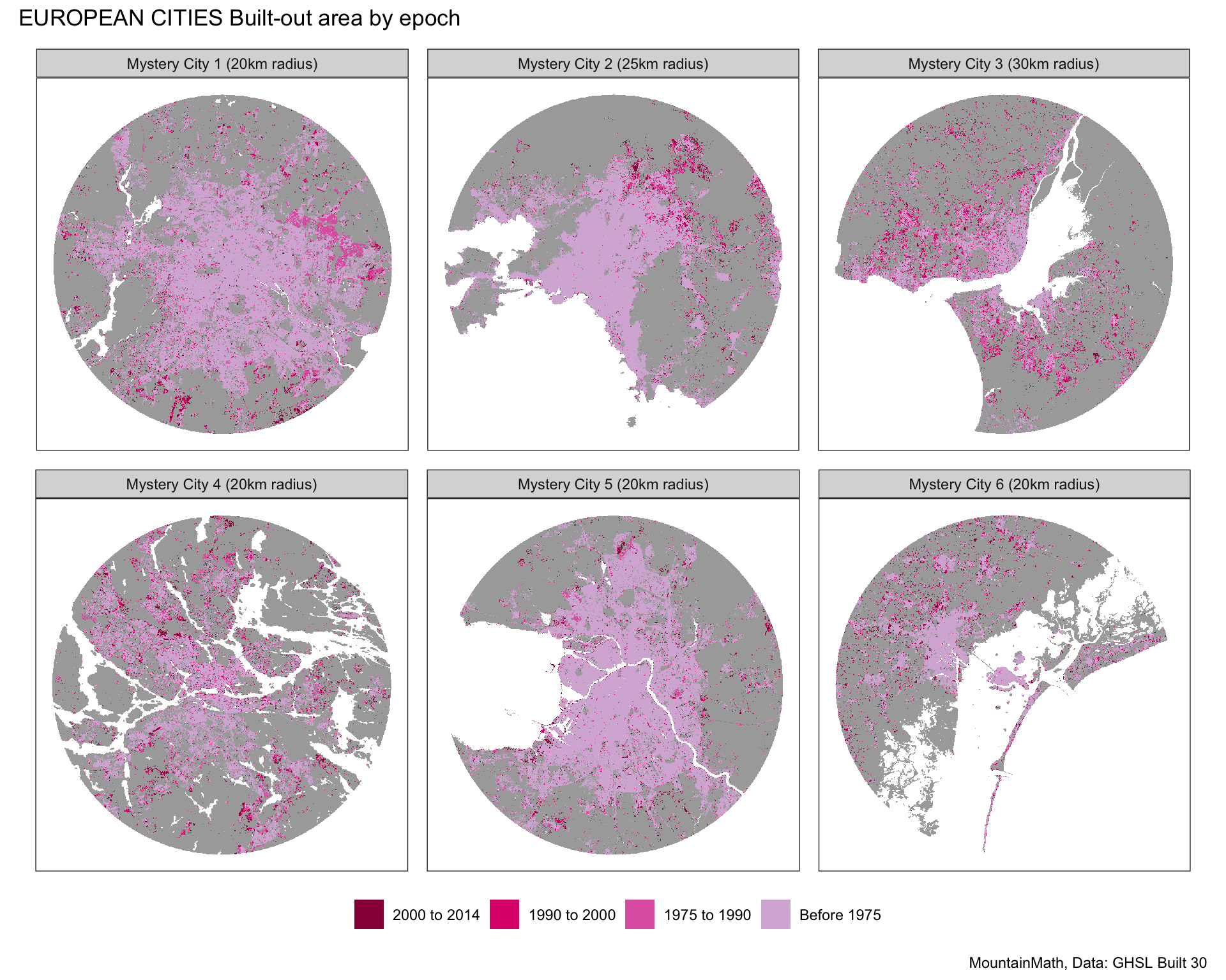
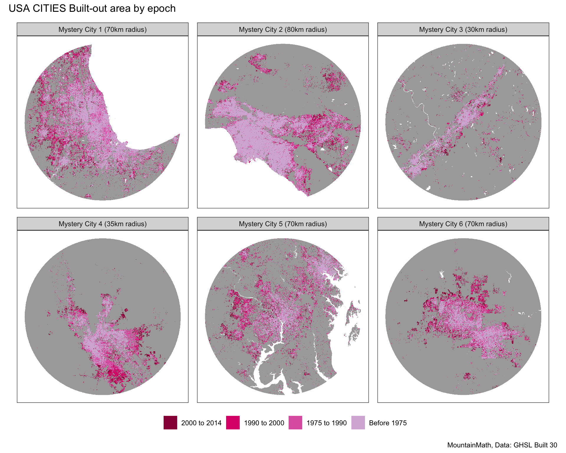
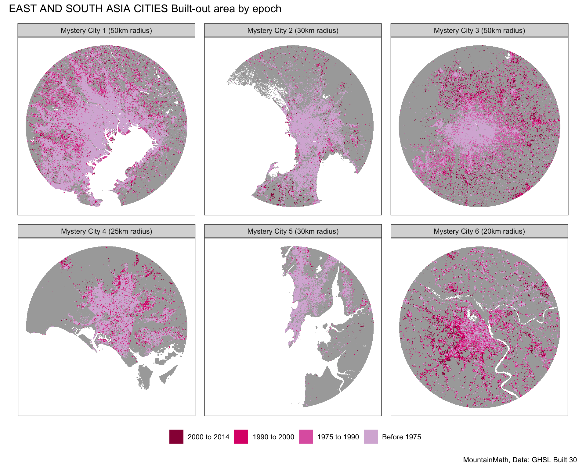
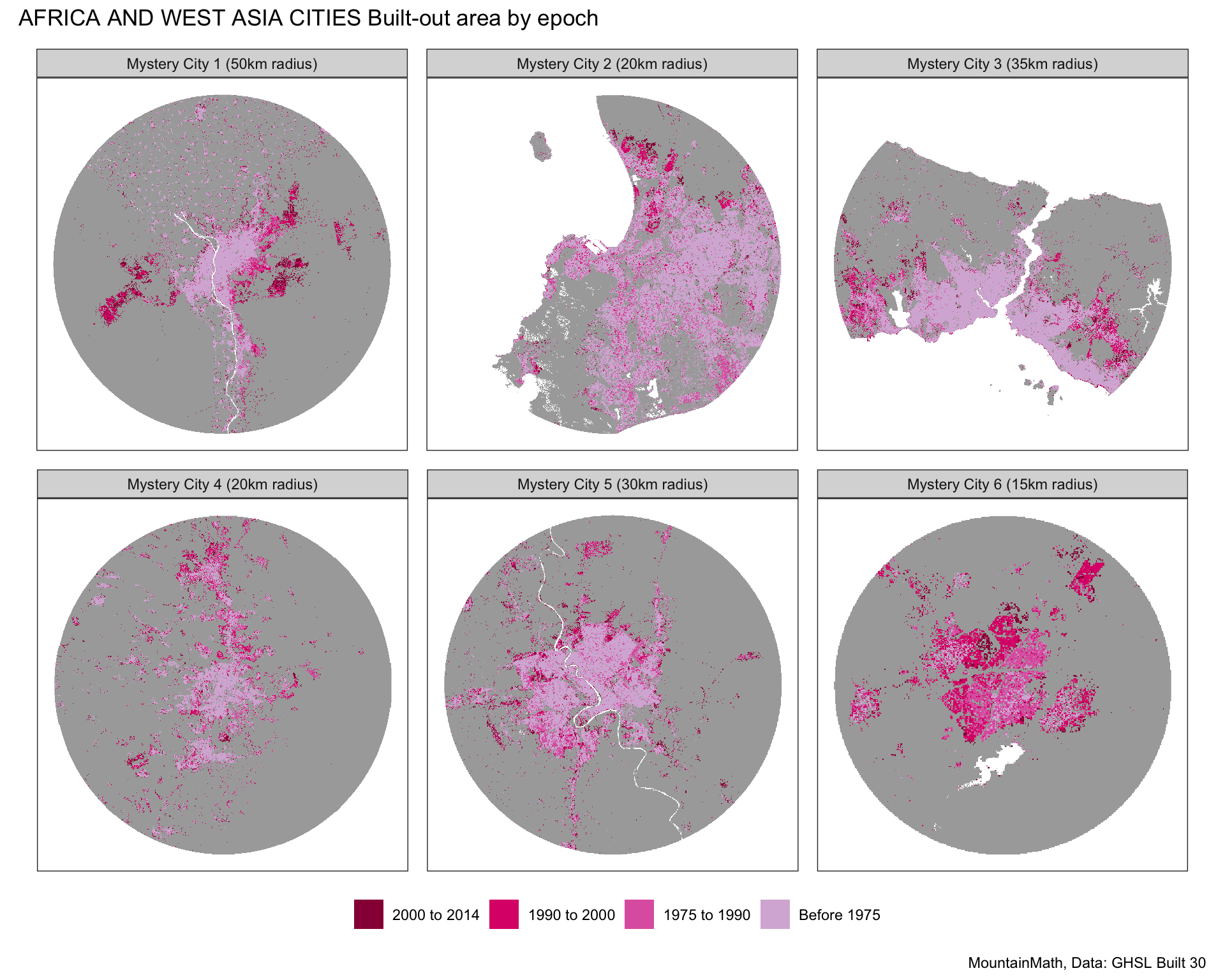
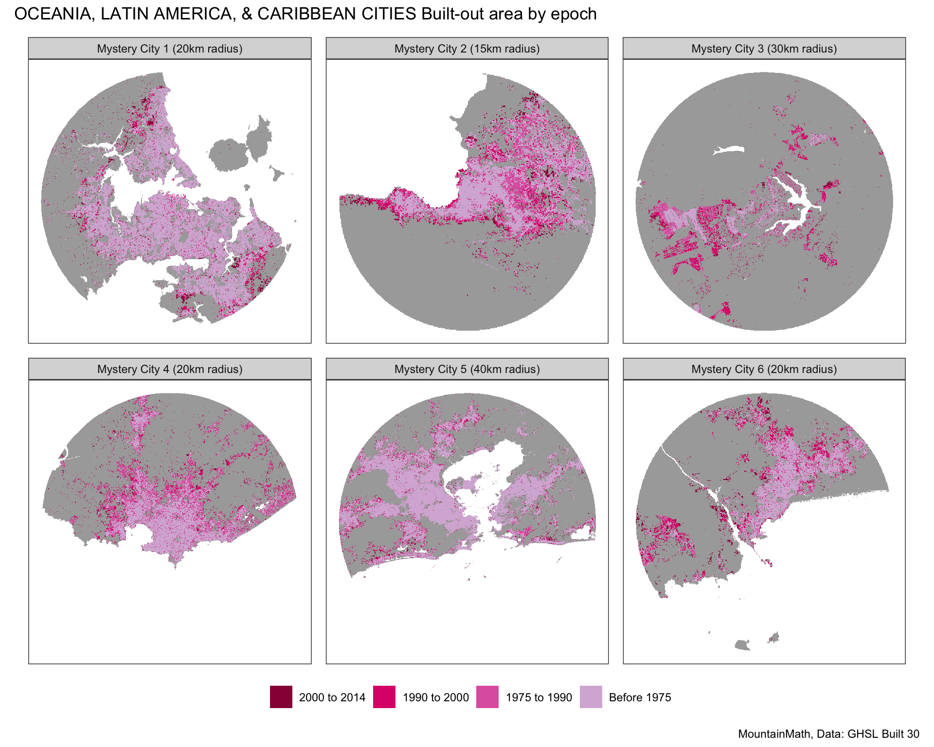
We can also play fun “Guess the City” games… Here’s the Canadian version.
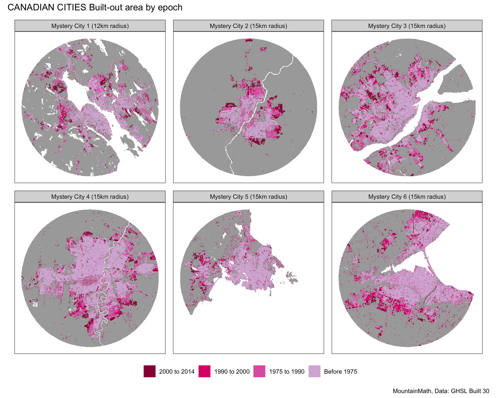
The Euro version.
USA. USA. USA.
Asia
Africa and Western Asia
Oceania, Latin America, & the Caribbean
Aside from having some fun, it’s also worth doing some checking to see how well the Landsat data works! We notice that a few of the cities we’ve looked at appear to have some of their built environment misclassified in terms of when it was built out. There are lots of potential sources of error, including, for instance, resolutions and image quality from 1975 satellites and how things like tree coverage and foliage might influence attempts to categorize land as built upon.
We’ll zoom in on two places we know relatively well, and have played with before: Vancouver and Minneapolis.
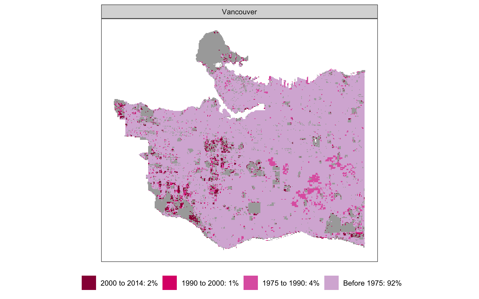
Here we’ve really zoomed in on the City of Vancouver. Overall it looks pretty good, which is to say Landsat estimations of built-out areas mostly fits with our expectations. But there are some weird bits, like wealthy and leafy parts of Shaughnessy, far west Point Grey, and the Southlands, that all look like they were recently developed. This might be explained by tree cover changes associated with redevelopment (and new mansion construction) in these areas. We can also see the recent construction of Champlain Heights in the SE corner of Vancouver, but this fits our priors insofar as the area famously remained undeveloped until the 1970s.
When we turn to Minneapolis what look like much larger misclassifications. Large parts of the central area of the city (e.g. Uptown near Lake Calhoun) are classified as being built up between 1975 and 1990.
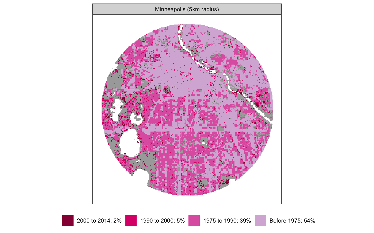
But experience, confirmed by a cross-check at a building age map of Minneapolis shows that almost all homes in these areas were built before 1970. In fact some pockets showing as solidly built up between 1975 and 1990 have homes almost exclusively built before 1910.
There are several possibly explanations for this misclassification. There is literature showing how difficult it is to train a classifier to deliver consistent results globally. A possible problem could have been dense tree cover that got thinned over the years, resulting in areas initially getting classified as undeveloped to later be classified as built-up, without much changes to what was on the ground. This could also happen because of better spatial resolution of Landsat satellites used for later years. That said, Minnesota was the worst example we found when browsing through various cities. (It’s addictive, we highly encourage grabbing the code and spending a couple of hours pointing it to different cities around the globe.)
Boomtown
We can find sprawl in well-established cities like Calgary and Edmonton, but the phenomenon becomes even more prominent when we look at cities that were quite small in 1975 and have experienced rapid growth since. The smaller boomtowns are where we can still watch how land gets eaten up for building more homes. Squamish provides a good example. Looking down from the top of the Chief it is hard not to notice the new development happening at the fringes, while the city centre seems to consist of more surface parking than buildings.
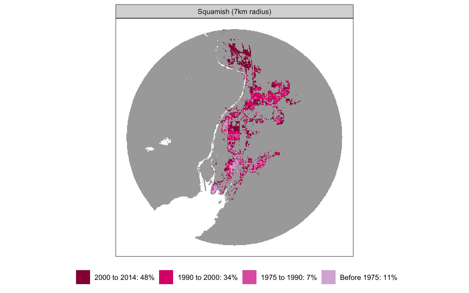
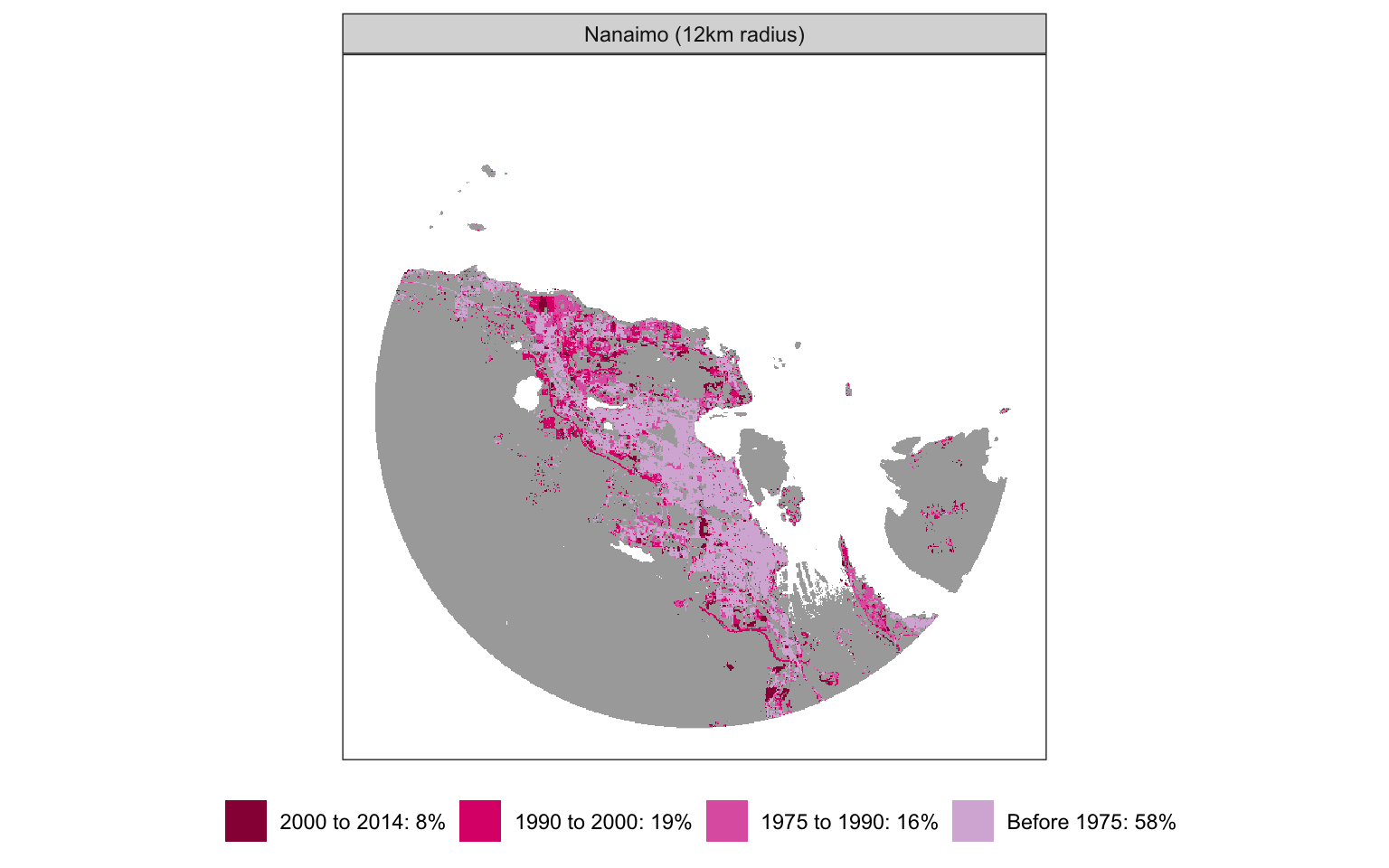
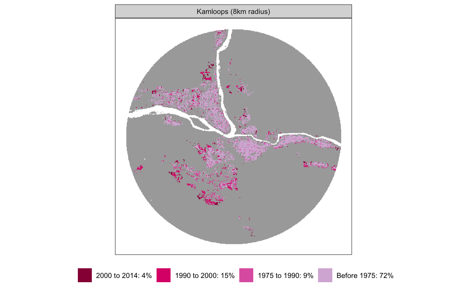
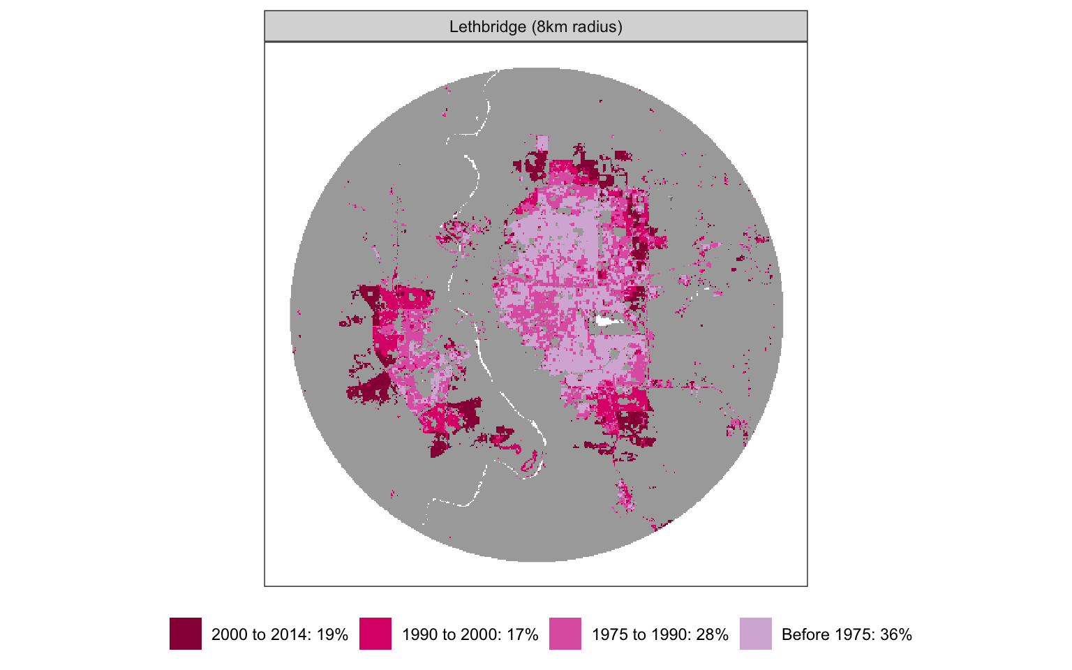
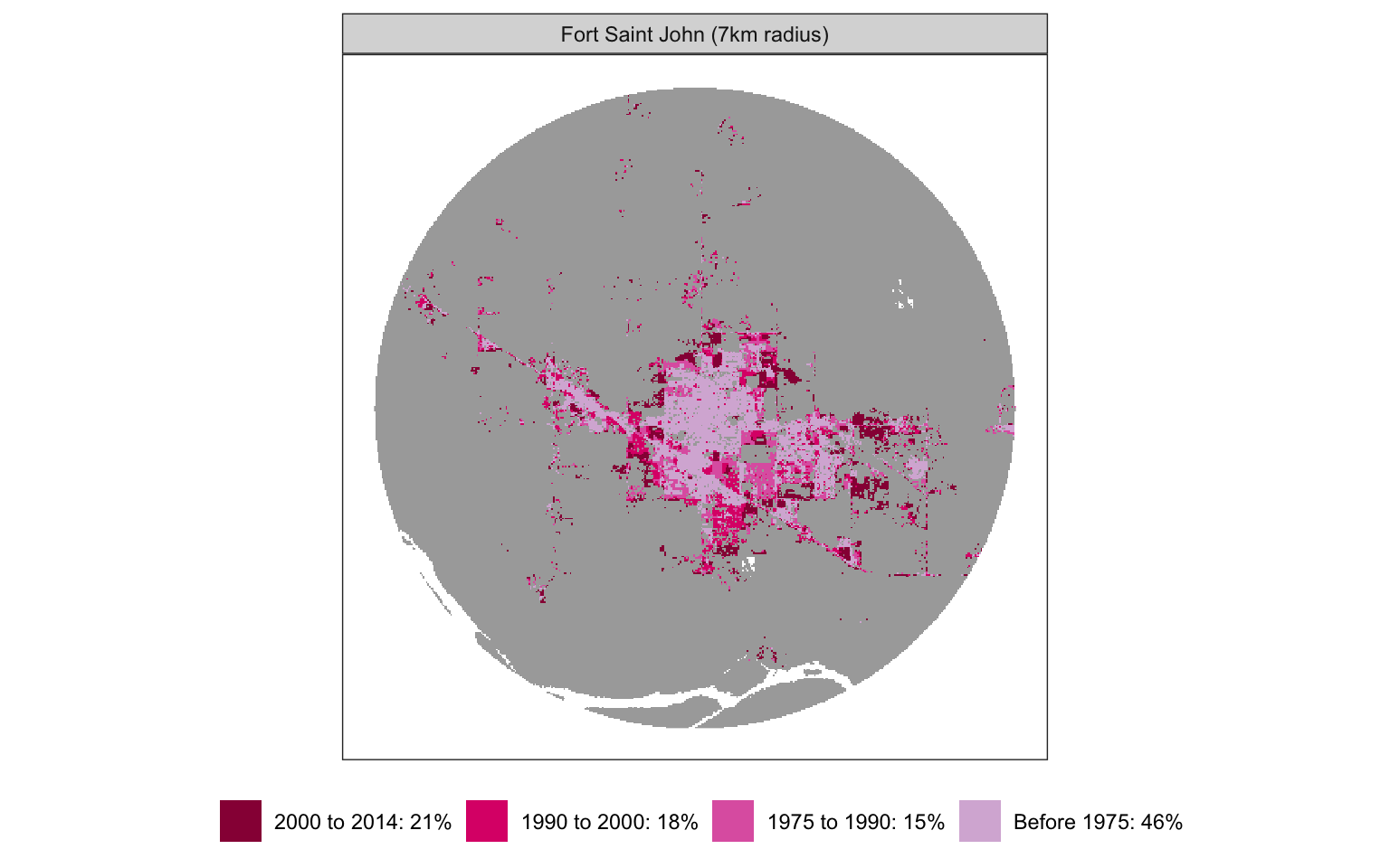
More City Six-Packs
Pulling down satellite data to look at patterns of historical urban sprawl is entirely too much fun. But we’re going to keep doing it. And while there are still some bugs to be worked out in terms of ground-truthing the satellite data, it mostly seems to provide a good approximation of the big picture for land use change. We’ll keep thinking through ways of understanding how different cities are growing, and returning to the real trade-offs in terms of reducing the footprint of growth.
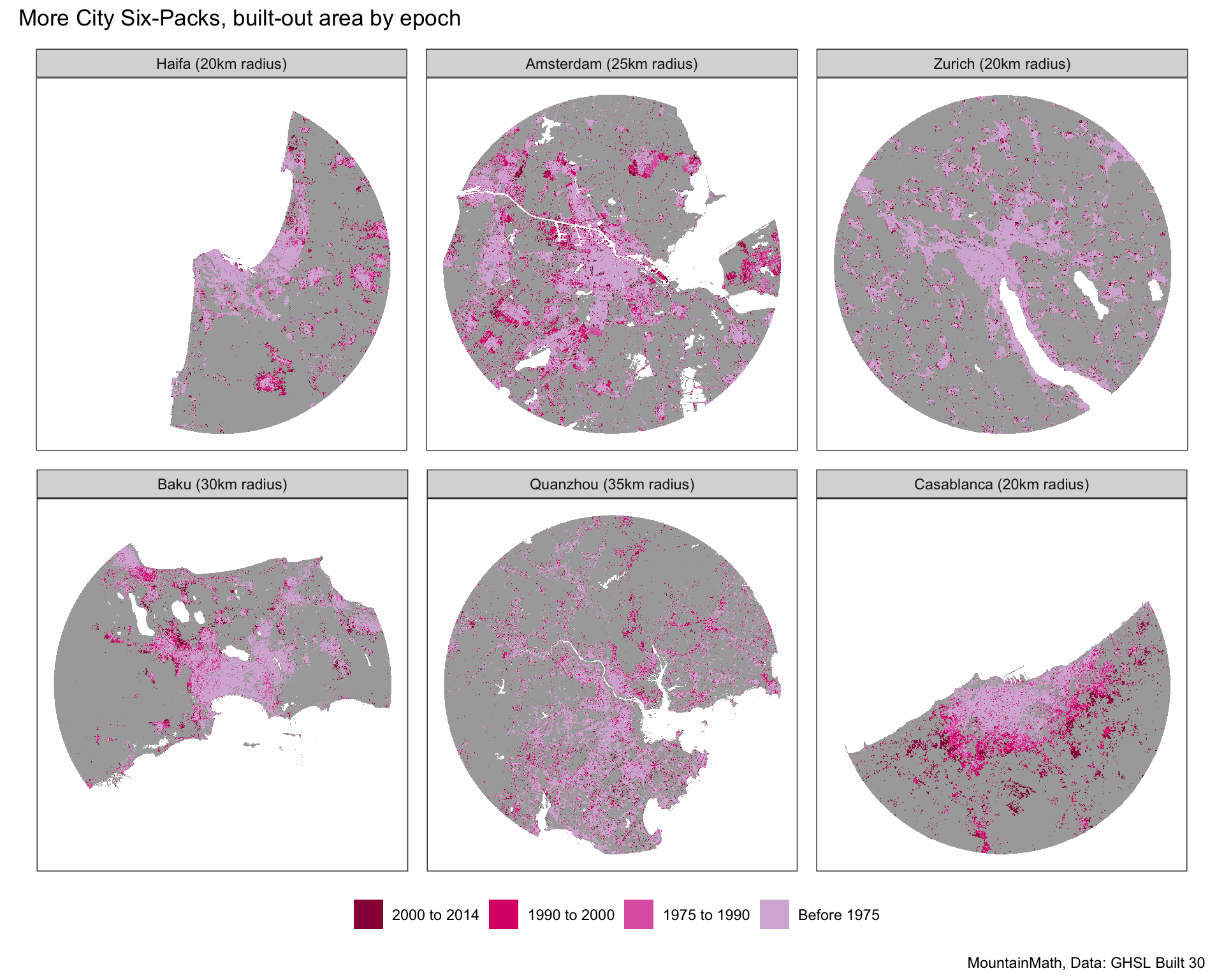
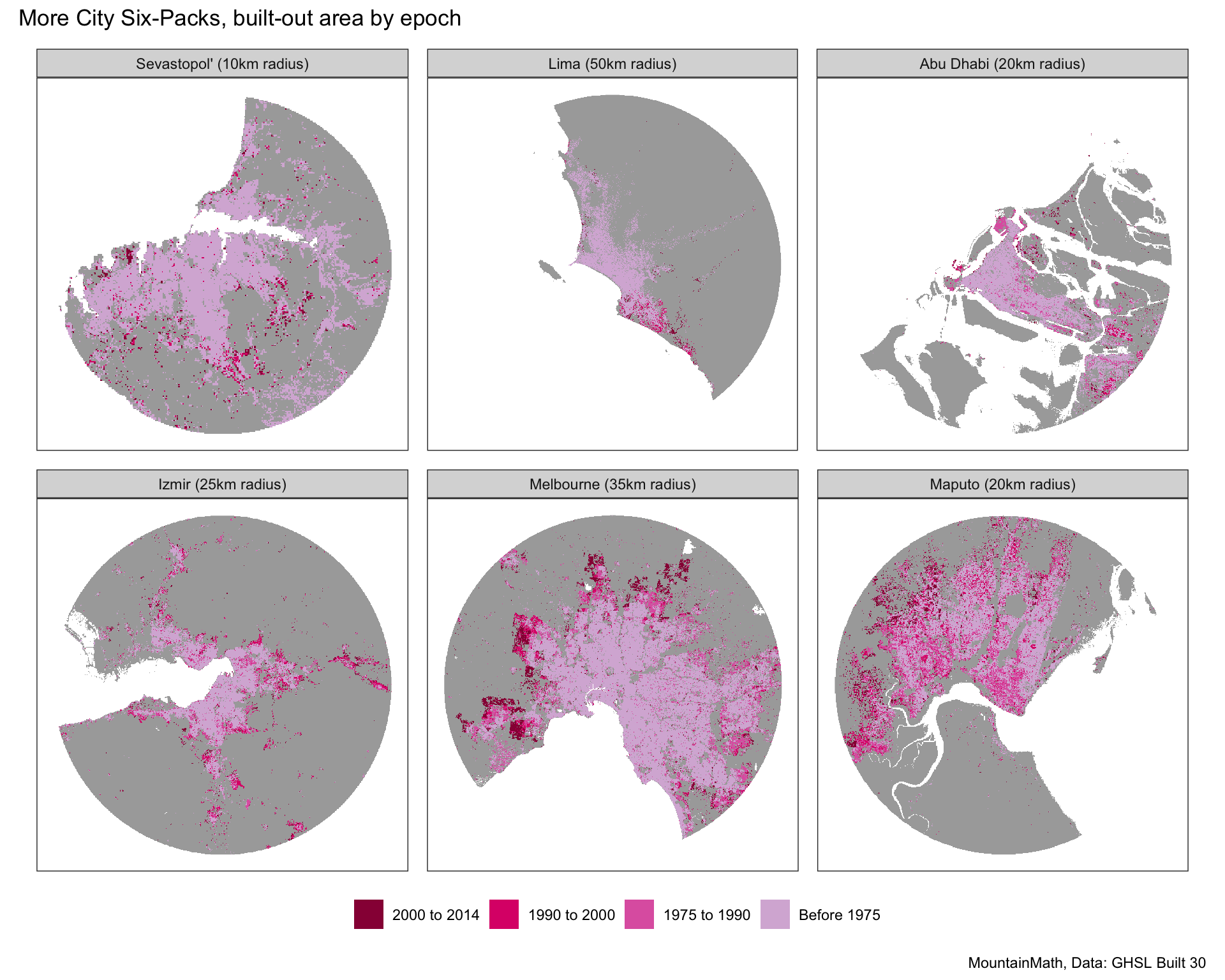
While we are at it, here are some more cities. (we can’t stop. send help!) For those that can’t wait to try out even more cities, the code for this post is available on GitHub for anyone to reproduce, adapt, or run their favourite cities.
Reproducibility receipt
## [1] "2021-08-22 18:40:16 PDT"## Local: master /Users/jens/Google Drive/R/mountaindoodles
## Remote: master @ origin (https://github.com/mountainMath/doodles.git)
## Head: [8ab33a5] 2021-08-21: city 6-packs## R version 4.1.0 (2021-05-18)
## Platform: x86_64-apple-darwin17.0 (64-bit)
## Running under: macOS Big Sur 10.16
##
## Matrix products: default
## BLAS: /Library/Frameworks/R.framework/Versions/4.1/Resources/lib/libRblas.dylib
## LAPACK: /Library/Frameworks/R.framework/Versions/4.1/Resources/lib/libRlapack.dylib
##
## locale:
## [1] en_CA.UTF-8/en_CA.UTF-8/en_CA.UTF-8/C/en_CA.UTF-8/en_CA.UTF-8
##
## attached base packages:
## [1] stats graphics grDevices utils datasets methods base
##
## other attached packages:
## [1] sf_1.0-2 patchwork_1.1.1 cityDensities_0.1.0
## [4] forcats_0.5.1 stringr_1.4.0 dplyr_1.0.7
## [7] purrr_0.3.4 readr_2.0.1 tidyr_1.1.3
## [10] tibble_3.1.3 ggplot2_3.3.3 tidyverse_1.3.1
##
## loaded via a namespace (and not attached):
## [1] Rcpp_1.0.7 lubridate_1.7.10 class_7.3-19 assertthat_0.2.1
## [5] digest_0.6.27 utf8_1.2.2 R6_2.5.1 cellranger_1.1.0
## [9] backports_1.2.1 reprex_2.0.0 evaluate_0.14 e1071_1.7-7
## [13] httr_1.4.2 blogdown_1.4 pillar_1.6.2 rlang_0.4.11
## [17] readxl_1.3.1 rstudioapi_0.13 jquerylib_0.1.4 rmarkdown_2.8
## [21] munsell_0.5.0 proxy_0.4-26 broom_0.7.6 compiler_4.1.0
## [25] modelr_0.1.8 xfun_0.24 pkgconfig_2.0.3 htmltools_0.5.1.1
## [29] tidyselect_1.1.1 bookdown_0.22 fansi_0.5.0 crayon_1.4.1
## [33] tzdb_0.1.2 dbplyr_2.1.1 withr_2.4.2 grid_4.1.0
## [37] jsonlite_1.7.2 gtable_0.3.0 lifecycle_1.0.0 DBI_1.1.1
## [41] git2r_0.28.0 magrittr_2.0.1 units_0.7-2 scales_1.1.1
## [45] KernSmooth_2.23-20 cli_3.0.1 stringi_1.7.3 fs_1.5.0
## [49] xml2_1.3.2 bslib_0.2.5.1 ellipsis_0.3.2 generics_0.1.0
## [53] vctrs_0.3.8 tools_4.1.0 glue_1.4.2 hms_1.1.0
## [57] yaml_2.2.1 colorspace_2.0-1 classInt_0.4-3 rvest_1.0.1
## [61] knitr_1.33 haven_2.4.1 sass_0.4.0Reuse
Citation
@misc{satellites-sprawl-and-city-six-packs.2021,
  author = {{von Bergmann}, Jens and Lauster, Nathan},
  title = {Satellites, {Sprawl,} and {City} {Six-Packs}},
  date = {2021-08-21},
  url = {https://doodles.mountainmath.ca/posts/2021-08-21-satellites-sprawl-and-city-six-packs/},
  langid = {en}
}
