<code>
library(tidyverse)
library(cansim)
library(cancensus)
library(dotdensity)
library(sf)
library(mountainmathHelpers)(Joint with Nathan Lauster and cross-posted at HomeFreeSociology)
library(tidyverse)
library(cansim)
library(cancensus)
library(dotdensity)
library(sf)
library(mountainmathHelpers)Are people liquids or solids?
Trick question: they’re kind of both. This matters in terms of how we track people and project their location forward in time. There are basic demographic methods that effectively take people as solids. We can see where they are now. We can see how they’ve been moving recently. We can age them forward in time, including adding new little people and imagining older people dying off. And we can project forward how many people we’ll have in the future.
But people are also liquid. They slosh around a bit, but they eventually tend to settle downhill into the places where there are containers for them. Here our best bet in terms of projecting people’s location forward in time is to figure out the lay of the land and where the most likely containers are going to be located.
Sometimes our liquid and solid projections match up ok. But other times they don’t. Let’s make this discussion a little more solid by zooming in to take a look at a potential divergence in projections right here in Metro Vancouver.
When - if ever - will suburban Surrey surpass the population of the City of Vancouver?
The solid answer to this question tends to be that it’s going to happen, and quite soon! The liquid answer is much less certain on this point, leaving it mostly contingent on how much housing gets built where.
We can see the answer to when Surrey will surpass the population of Vancouver in recently released StatCan population projections at the municipal (census subdivision) level. StatCan’s method, in a nutshell, treats people as solid, aging them forward in place (within CSDs) via a crude approximation from past trends and made to sum into earlier calculated projections across the broader region (CD). Past net migration enters into past trends by age group and becomes extrapolated into the future. In trying to avoid running into absurd scenarios like negative population or unrealistically large growth scenarios in select areas and subgroups they crudely extrapolate areas and age groups that historically have been growing linearly and those that have been declining exponentially (while using language that would make any high school math teacher tear their hair out, but never mind that). More holistically this could be dealt with by a mechanism that implements regression to the mean over time.
We can see a slightly different answer to when Surrey will surpass the population of Vancouver in more standard provincial projections released by BC Stats in British Columbia. BC Stats also treats people as solids, but applies more refined methods to projecting age cohorts forward based upon distinct components of change (fertility, mortality, and migration) estimated from the past with some adjustments for current policies and future expectations, especially concerning immigration.
Figure 1 shows both of these projections, for BC Stats, the cross-over where Surrey surpasses Vancouver is imminent, happening sometime just after the Census, by the end of 2026. For StatCan, it looks like it’s one year further away, happening by the end of 2027.
metro_van_cities <- list_census_regions("2021") |>
  filter(level=="CSD",CMA_UID=="59933") |>
  add_unique_names_to_region_list() |>
  mutate(Name=fct_reorder(Name,-coalesce(pop,0))) |>
  select(GeoUID=region,Name)

bc_projections <- read_csv(here::here("data/Population_Projections_metro_van.csv"),skip=6) |>
  pivot_longer(matches("_\\d{4}$"),names_pattern=c("(.+)_(\\d{4})"),names_to=c("Series","Year"),values_to="Population") |>
  mutate(Name=gsub(", District Municipality", " (DM)",Municipality) |>
           gsub(", City of", " (CY)", x=_)) |>
  mutate(Date=as.Date(paste0(Year,"-01-01"))) |>
  select(Date,Municipality,Name,Series,Population) |>
  left_join(metro_van_cities,by="Name") |>
  select(-Name) |>
  left_join(metro_van_cities,by="GeoUID") |>
  mutate(Series=recode(Series,"Estimate"="Estimates",
                       "Projection"="Projections"))

csd_estimates <- get_cansim_connection("17-10-0155", refresh="auto") |>
  filter(substr(GeoUID,1,4) == "5915",
         nchar(GeoUID)==7) |>
    collect_and_normalize(default_month = "01") |>
  left_join(metro_van_cities,by="GeoUID")

csd_projections <- get_cansim_connection("17-10-0162", refresh="auto") |>
    filter(Gender=="Total - gender",
           `Age group`=="All ages",
           `Projection scenario`=="Projection scenario M1: medium-growth",
            substr(GeoUID,1,4) == "5915",
            nchar(GeoUID)==7) |>
    collect_and_normalize(default_month = "01") |>
  left_join(metro_van_cities,by="GeoUID")


all_data <- bind_rows(
    csd_projections |> mutate(Series="StatCan projections"),
    csd_estimates |> mutate(Series="Statcan estimates")
  ) |>
  mutate(Source="StatCan") |>
  rename(Population=val_norm) |>
  bind_rows(bc_projections |> mutate(Source="BC Stats") |> filter(Series=="Projections"|Date=="2024-01-01") |>
              mutate(Series="BC Stats projections")) |>
  mutate(Series=factor(Series,levels=c("Statcan estimates","StatCan projections","BC Stats projections")))

all_data_cleaned  <- all_data %>%
  filter(Name %in% ((.) |> count(Name,Series) |> count(Name) |> filter(n==3) |> pull(Name)))

line_types <- setNames(c("solid","dashed","dotted"),
                           c("Statcan estimates","StatCan projections","BC Stats projections"))
source_colours <- setNames(sanzo::trios$c157,
                           c("Statcan estimates","StatCan projections","BC Stats projections"))

all_data_cleaned |>
  filter(Name %in% c("Vancouver","Surrey")) |>
  filter(Date>="2015-01-01",Date<="2035-01-01") |>
ggplot(aes(x=Date, y=Population, color=Series,linetype=Name)) +
    geom_line(linewidth = 1) +
    geom_point(shape=21) +
  scale_colour_manual(values=source_colours) +
  scale_x_date(date_breaks = "5 years", date_labels = "Jul %Y") +
  scale_y_continuous(labels=\(x)scales::comma(x,scale=10^-3,suffix="k"),
                     trans="log", breaks=seq(500,900,50)*1000) +
    labs(title="Population Estimates and Projections for Vancouver and Surrey",
         x=NULL,
         y="Population",
         linetype="Muncipality",
colour="Source") 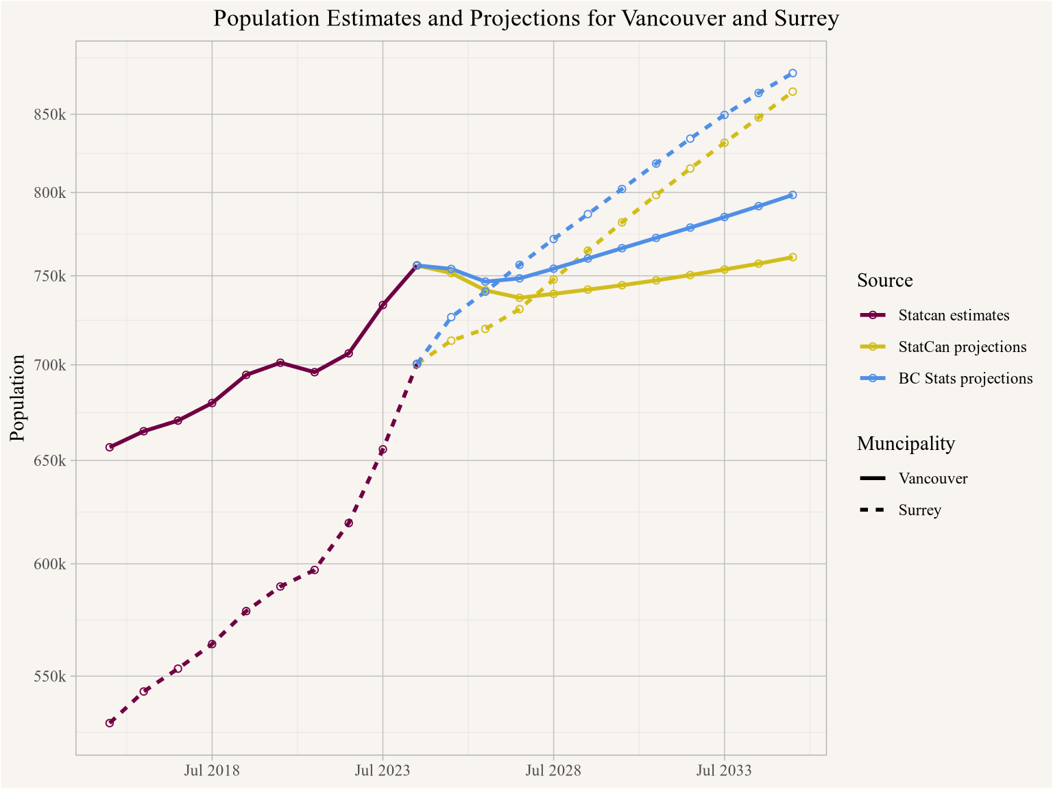
We can see the cross-over between Vancouver and Surrey is heavily driven by the projected decline in Vancouver’s population. This is striking. Where does it come from? As it turns out, temporary residents arriving in the metro area of Vancouver have more often landed in the City of Vancouver than the City of Surrey. Recent rollbacks in temporary residents due to Canadian immigration policy have been extrapolated forward, and have been built into the solid population models of both StatCan and BC Stats, where they enter in just slightly different ways. The assumption is that if you turn off this conveyor belt of temporary residents, then the City of Vancouver’s population will decline more than the City of Surrey’s. But is this correct? We could work with different assumptions. Let’s think about our conveyor belt as more like a stream, one of many feeding the pond of our metropolitan area. What happens to the deepest part of the pond - our central city - if this particular stream gets diverted?
Where will people sloshing around Metro Vancouver land? As it turns out, they land mostly where there’s housing to contain them. If we believe this, then projecting in the future should be based mostly on where housing is likely to land rather than our cohort projections. To make this more concrete, let’s think about housing growth.
Overall, both Vancouver and Surrey have been adding housing in recent years. To better match housing to population we would want to look more broadly at housing services provided, not just number of housing units. We don’t have open data on square footage or number of bedrooms added, but we can use dwelling types, combined with household size estimates for each dwelling type, to derive a rough and imperfect measure of growth in housing capacity and relate the to population growth. We show the household size by type estimates derived from the 2021 census in Table 1.
dwelling_types <- c("Single", "Semi-Detached", "Row", "Apartment")

hhsize_data <- get_cansim_connection("98-10-0240") |>
  filter(GeoUID %in% c("5915022","5915","5915004"),
         `Household size (8)` %in% c("Average household size","Total - Household size"),
         `Number of bedrooms (6)`=="Total - Number of bedrooms",
         `Statistics (3C)`=="Number of private households") |>
  collect_and_normalize() |>
  filter(`Tenure (4)`=="Total - Tenure") |>
  select(GeoUID,value=VALUE,`Dwelling Type`=`Structural type of dwelling (10)`,name=`Household size (8)`) |>
  pivot_wider(names_from=name,values_from=value) |>
  filter(`Dwelling Type` !="Total - Structural type of dwelling") |>
  mutate(`Dwelling Type`=recode(`Dwelling Type`,
                                "Single-detached house"="Single",
                                "Semi-detached house"="Semi-Detached",
                                "Row house"="Row",
                                "Apartment in a building that has fewer than five storeys"="Apartment",
                                "Apartment in a building that has five or more storeys"="Apartment")) |>
  summarise(hhsize=weighted.mean(`Average household size`,`Total - Household size`),.by=c(GeoUID,`Dwelling Type`)) |>
  filter(`Dwelling Type` %in% dwelling_types) |>
  mutate(`Dwelling Type`=factor(`Dwelling Type`,levels=dwelling_types))

hhsize_data |>
  left_join(metro_van_cities, by="GeoUID") |>
  mutate(Name=coalesce(Name,"Metro Vancouver")) |>
  select(-GeoUID) |>
  arrange(`Dwelling Type`) |>
  mutate(hhsize=round(hhsize,1)) |>
  pivot_wider(names_from=`Dwelling Type`,values_from=hhsize) |>
tinytable::tt()| Name | Single | Semi-Detached | Row | Apartment |
|---|---|---|---|---|
| Metro Vancouver | 3.1 | 2.7 | 2.8 | 1.9 |
| Vancouver | 2.9 | 2.7 | 2.6 | 1.7 |
| Surrey | 3.4 | 2.6 | 2.9 | 2.3 |
Dwellings of most types tend to contain more people in Surrey than in Vancouver. This likely reflects roomier dwellings in Surrey, indicating greater housing services being provided on average per dwelling, though it’s possible differences are also picking up other patterns, like more doubling up. Overall, our basic assumption is that on average dwellings produced in Surrey will probably contain slightly more of our liquid people than in the City of Vancouver. Multiplying these figures with our data on recent completions (with a minor adjustment for demolitions), we can roughly estimate the net housing capacity recently added per year in Vancouver and Surrey. The resulting estimated housing capacity growth is shown next to StatCan estimated population growth in Figure 2.
summarize_annual_by_type <- function(data){
  data |>
    filter(`Dwelling Type`!="All") |>
    mutate(Year=strftime(Date %m+% months(6),"%Y")) |>
    summarize(Total=sum(Value,na.rm=TRUE),
              months=n(),.by=c(`Dwelling Type`,Year)) |>
    filter(months==12) |>
    select(-months)
}

van_completions <- cmhc::get_cmhc(survey = "Scss", series = "Completions", dimension = "Dwelling Type", breakdown = "Historical Time Periods", geo_uid = "5915022") |>
  summarize_annual_by_type()

surrey_completions <- cmhc::get_cmhc(survey = "Scss", series = "Completions", dimension = "Dwelling Type", breakdown = "Historical Time Periods", geo_uid = "5915004") |>
  summarize_annual_by_type()

yvr_completions <- cmhc::get_cmhc(survey = "Scss", series = "Completions", dimension = "Dwelling Type", breakdown = "Historical Time Periods", geo_uid = "59933") |>
  summarize_annual_by_type()


demolition_fudge <- 0.93

completions_combined <- bind_rows(
  van_completions |> mutate(GeoUID="5915022"),
  surrey_completions |> mutate(GeoUID="5915004"),
  yvr_completions |> mutate(GeoUID="5915")
) |>
  left_join(hhsize_data,by=c("GeoUID","Dwelling Type")) |>
  summarize(change=sum(Total*demolition_fudge*hhsize),.by=c(GeoUID,Year)) |>
  mutate(Metric="Housing capacity growth")

pop_combined <- bind_rows(
  get_cansim_connection("17-10-0155", refresh="auto") |>
    filter(GeoUID %in% c("5915022","5915004")) |>
    collect_and_normalize(default_month = "01"),
  get_cansim_connection("17-10-0152", refresh="auto") |>
    filter(GeoUID %in% c("5915"),
           `Age group`=="All ages",
           Gender=="Total - gender") |>
    collect_and_normalize(default_month = "01")
  )|>
  select(Year=REF_DATE,GeoUID,Population=val_norm) |>
  mutate(change=Population - lag(Population, order_by = Year),.by=GeoUID) |>
  select(-Population) |>
  mutate(Metric="Population growth") |>
  filter(!is.na(change))


bind_rows(pop_combined,
          completions_combined,) |>
  filter(Year>=2002) |>
ggplot(aes(x=as.integer(Year), y=change, color=Metric)) +
  geom_line() +
  facet_wrap(~GeoUID,scales="free_y",
             labeller=as_labeller(c("5915"="Metro Vancouver","5915022"="City of Vancouver",
                                    "5915004"="City of Surrey"))) +
  geom_point(shape=21) +
  scale_color_manual(values=sanzo::duos$c085) +
  theme(legend.position = "bottom") +
  scale_y_continuous(labels=\(x)scales::comma(x)) +
    labs(title="Population vs Housing Capacity Growth",
         x=NULL,
         y="Number of people",
         color=NULL,
         caption="CMHC Scss and StatCan Tables 17-10-0152, 17-10-0155, 98-10-0240")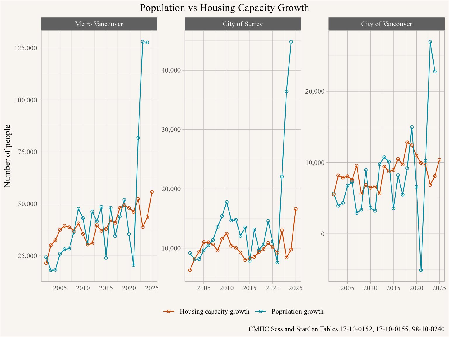
The relationship is spiky and imperfect, reflecting in part the crudeness of our estimation as well as the compressibility of liquid demographics exhibiting short term adjustments in household formation and doubling up to smooth out mismatches. But generally as we add more housing, we also add more population. This relationship holds up pretty well until COVID hits in 2020. By 2021, the population of the City of Vancouver dropped in spite of additions to housing. Multiple issues account for this shift: immigrants stopped arriving, universities and workplaces went remote, and people increasingly valued more room at home (for work-from-home offices) relative to proximity to downtown. This last factor likely accounts for some of suburban Surrey’s resilience. Bigger homes and fewer commutes changed the landscape of demand. But people are liquid, and slosh, slosh, you’ll never guess what happened next. Lots of people sloshed back again!
This sloshing is important. Like a tsunami, the rollback in the City of Vancouver was temporary, to be followed by an inundation that completely erased the previous year’s loss in population in the City. What limited the City of Vancouver’s growth at that point? Housing. There was only so much available. People could double up (and they did!), exceeding the growth rate in housing capacity. But otherwise people would have to find room in the suburbs, which they also did. We can see from Surrey’s population that it also boomed. Surrey also saw lots of doubling up, but the boom there was further facilitated by a stronger underlying boost to housing capacity than we saw in the City of Vancouver.
Which brings us back to the differences between liquid and solid demographics. In a liquid demography, people will slosh around, but eventually make their way toward settling in the housing that’s available in the places they want to live. There are limits to how many people can be added, but we have a rough idea where they want to be. Accordingly, we need to pay attention mostly to how much supply has been created to meet the landscape of demand. And we don’t want to take housing for granted! In a solid demography, especially one where we don’t even put people in households but just focus on age cohorts, housing and its constraints are effectively ignored.
Ideally we want to bring liquid and solid treatments of people together. Both population dynamics and housing constraints matter. (Mulder 2006) Because it is the case that housing doesn’t always get filled up. Just like housing doesn’t magically appear in response to population change, people don’t suddenly appear in response to additions to housing supply. But ignoring housing constraints is especially problematic when we’re using population projections to estimate how much housing we need. More on that below!
Let’s get back to the horse race between Vancouver and Surrey. In terms of projecting when (or if) Surrey will overtake Vancouver in population, the liquid demography asks first, who is building more housing? Then, how is the landscape of demand changing? And finally, just as a check, are there any good reasons to believe we’ll see housing left empty even when people want to live there?
Figure 3 provides information on who is building more housing. Here “completions” refer to what’s just been added, with “starts” and “under construction” telling us what’s coming down the pipeline. In general, we’d expect completions to lag starts, but note the rise in “under construction” visible in both cities, which reflects increasingly lengthy construction timelines, reducing the predictability for when things will finish. (von Bergmann 2017b)
van_sur_completions <- metro_van_cities |>
  filter(grepl("^Vancouver|Surrey",Name)) |>
  pull(GeoUID) |>
  map_dfr(\(geo) {
    c("Starts","Completions") |>
      map_dfr(\(series) {
        cmhc::get_cmhc(survey = "Scss", series = series, dimension = "Dwelling Type",
                       breakdown = "Historical Time Periods", geo_uid = geo) |>
      summarize_annual_by_type() |>
      mutate(Series=series)
      }) |>
      bind_rows(
               cmhc::get_cmhc(survey = "Scss", series = "Under Construction", dimension = "Dwelling Type",
                       breakdown = "Historical Time Periods", geo_uid = geo) |>
                 filter(strftime(Date,"%m")=="07") |>
                 mutate(Year=strftime(Date,"%Y"),
                        Series="Under Construction") |>
                 select(`Dwelling Type`, Year , Total=Value, Series, GeoUID)
      ) |>
      mutate(GeoUID=geo)
  }) |>
  left_join(metro_van_cities,by="GeoUID")

van_sur_completions |>
  ggplot(aes(x=as.integer(Year),y=Total,fill=fct_rev(`Dwelling Type`))) +
  geom_col(position="stack") +
  facet_grid(Series~Name, scales="free_y") +
  scale_y_continuous(labels=scales::comma) +
  theme(legend.position = "bottom") +
  #scale_fill_manual(values=sanzo::duos$c114, guide="none") +
  labs(title="Housing construction in Vancouver and Surrey",
       x=NULL,
       y="Number of units",
       fill=NULL,
       caption="CMHC Scss")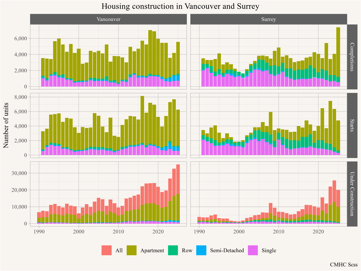
We can see 2025 was a very good year for Surrey completions. But historically Vancouver has been building more dwelling units, and its pipeline looks much more robust. Still, as we have noted Vancouver’s dwellings have generally been smaller. We don’t have good historical open data on number of bedrooms, but we can continue to proxy for that by breaking data out by dwelling type. Importantly, Surrey is starting to run out of room for greenfield development due to the Agricultural Land Reserve, and it’s increasingly building rowhouses and apartments instead. New single-family detached dwellings built in Surrey are going to look increasingly like those built in Vancouver - either replacing a tear-down, in which case they don’t contribute much to supply, or laneway homes, which generally accommodate fewer people.
At the same time the City of Vancouver has several planning initiatives that look at loosening up regulation to allow more apartments in several key areas; the Broadway Corridor, Heather Lands, Jericho Lands, the Villages initiative and others. This includes plans to densify around Skytrain stations. Of course, this also applies to Surrey, but demand is much higher in the City of Vancouver, as can be seen by looking at the modelled price surface for multiplexes from our report on the provincial SSMUH and TOA initiatives. (von Bergmann et al. 2023)
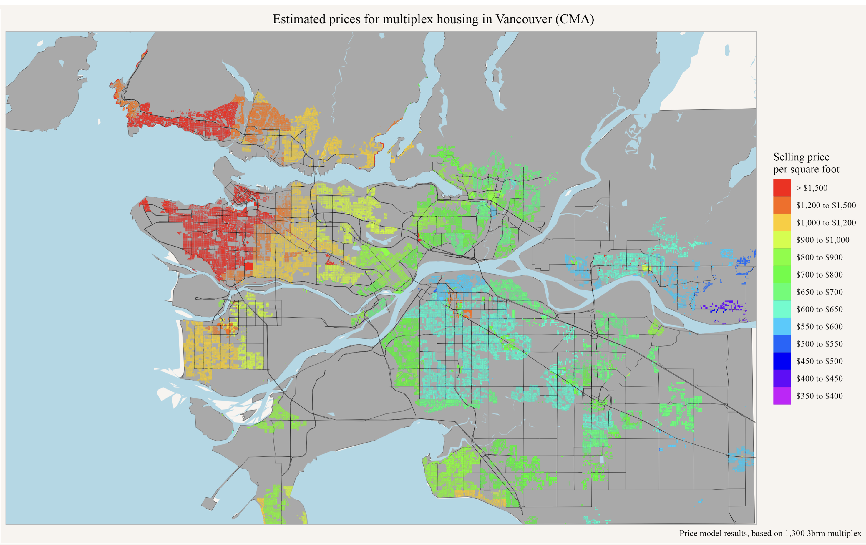
The price surface in Figure 4 provides a glimpse at the underlying landscape of desire. Residential space in Surrey is painted in blue and green, at much lower price points than the same space in Vancouver, neatly split between the red of Westside and orange of Eastside. People seem to generally want to move toward downtown Vancouver. What holds them back? Primarily the lack of housing. Similarly, CMHC’s report on supply constraints highlights spatial differential in unmet demand for housing within Metro Vancouver. (CMHC 2018) This kind of landscape suggests to a liquid demographer that if you divert one set of streams toward downtown Vancouver, like non-permanent resident inflows, they’re most likely going to be replaced by other streams that were also headed in that direction, but got backed up to places like Surrey by the competition for limited container space.
Figure 5 gives another view into this by showing workers by whether they commute within our outside of their city of residence on their way to work.
commute_data <- get_census("2021",regions=list(CMA="59933"), level="DA",
                           vectors=c(workers="v_CA21_7617",same_csd="v_CA21_7620"),
                           geo_format="sf") |>
  mutate(different_csd=pmax(0,workers - same_csd)) |>
  mutate(van_sur=CSD_UID %in% c("5915022","5915004")) |>
  mutate(across(c(different_csd,same_csd), ~replace_na(.,0)))


random_round <- function(x) {
    v <- as.integer(x)
    r <- x-v
    test <- stats::runif(length(r), 0.0, 1.0)
    add=rep(as.integer(0),length(r))
    add[r>test] <- 1L
    value <- v+add
    value <- ifelse(is.na(value) | value<0,0,value)
    return(value)
}


scale <- 50
commute_data <- commute_data %>%
      dplyr::mutate(across(c(different_csd,same_csd),~(./scale))) %>%
      dplyr::mutate(across(c(different_csd,same_csd),random_round))

all_data <- c("same_csd","different_csd") |>
  lapply(\(cat) {
    dd <- commute_data |>
      filter(!!as.name(cat)>0)
    st_sample(dd,size=dd |> pull(cat),
              warn_if_not_integer=FALSE) |>
      st_as_sf() |>
      mutate(Type=cat)
  }) |>
  bind_rows() %>%
  slice_sample(.,n=nrow(.), replace = FALSE) |>
  mutate(Type=recode(Type,
                     "same_csd"="Same city",
                     "different_csd"="Different city"))

cov_sur_geo <- get_census("2021",regions=list(CSD=c("5915022","5915004")),geo_format="sf")

ggplot(all_data) +
  geom_water() +
  #geom_roads() +
  geom_sf(aes(colour=Type),size=0.5, alpha=0.5) +
  geom_sf(data=cov_sur_geo,fill=NA,linewidth=1) +
  coord_bbox(metro_van_bbox("tight")) +
  theme(legend.position="bottom") +
  guides(colour=guide_legend(override.aes=list(size=2,alpha=1))) +
  scale_colour_manual(values=sanzo::duos$c079) +
  annotate("text",x=-123.25,y=49.3,label="Vancouver",size=4,color="black") +
  annotate("curve",x=-123.25,xend=-123.12,y=49.29,yend=49.25,
           curvature=0.2,linewidth=0.75,
           arrow=arrow(length=unit(0.3,"cm")),color="black") +
  annotate("text",x=-122.95,y=49.05,label="Surrey",size=4,color="black") +
  annotate("curve",x=-122.95,xend=-122.82,y=49.06,yend=49.13,
           curvature=0.2, linewidth=0.75,
           arrow=arrow(length=unit(0.3,"cm")),color="black") +
  labs(title="Place of work status in Metro Vancouver",
       colour="Place of work",
       x=NULL,y=NULL,
       caption="StatCan census 2021")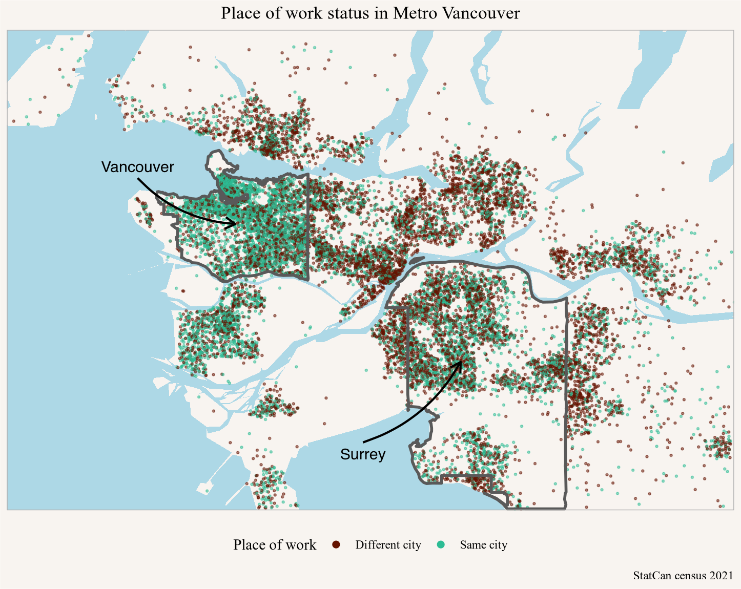
commute_flow_lookup <- get_cansim_connection("98-10-0459") |>
  filter(substr(GeoUID,1,4) == "5915",
         nchar(GeoUID)==7) |>
  select(GeoUID,GEO) |>
  distinct() |>
  collect()

metro_names <- list_census_regions("2021") |>
  filter(level=="CSD",CMA_UID=="59933") |>
  add_unique_names_to_region_list() |>
  select(GeoUID=region,Name)

por_lookup <- get_cansim_column_categories("98-10-0459","Place of residence") |>
  mutate(id=Hierarchy,UID=gsub("\\[|\\]","",`Classification Code`)) |>
  select(id,UID)

pow_lookup <- get_cansim_column_categories("98-10-0459","Place of work") |>
  select(id=`Member ID`,Name=`Member Name`) |>
  left_join(por_lookup, by=c("id"="id"))

yvr_sur_por <- pow_lookup |>
  filter(UID %in% c("5915022","5915004"))

workers <- get_cansim_connection("98-10-0459") |>
  filter(GeoUID %in% c("5915022","5915004")) |>
  collect_and_normalize() |>
  filter(`Gender (3)`=="Total - Gender") |>
  summarize(Workers=sum(VALUE),.by=c(GeoUID)) |>
  left_join(metro_names, by="GeoUID")

jobs <- get_cansim_connection("98-10-0459") |>
  filter(`Place of work` %in% yvr_sur_por$Name) |>
  collect_and_normalize() |>
  filter(`Gender (3)`=="Total - Gender") |>
  summarize(Workers=sum(VALUE),.by=c(`Place of work`)) |>
  left_join(yvr_sur_por, by=c("Place of work"="Name")) |>
  left_join(metro_names, by=c("UID"="GeoUID"))

flows <- get_cansim_connection("98-10-0459") |>
  filter(GeoUID %in% c("5915022","5915004")) |>
  filter(`Place of work` %in% yvr_sur_por$Name) |>
  collect_and_normalize() |>
  filter(`Gender (3)`=="Total - Gender") |>
  left_join(metro_names |> select(Origin=Name,GeoUID), by=c("GeoUID")) |>
  left_join(yvr_sur_por |> select(`Place of work`=Name,UID), by="Place of work") |>
  left_join(metro_names |> select(Destination=Name,UID=GeoUID), by="UID") |>
  select(Origin,Destination,Value=VALUE)

van_sur_commuters <- flows |>
  filter(Origin=="Vancouver",Destination=="Surrey") |> pull(Value)
sur_van_commuters <- flows |>
  filter(Origin=="Surrey",Destination=="Vancouver") |> pull(Value)

van_workers <- workers |>
  filter(Name=="Vancouver") |>
  pull(Workers)
sur_workers <- workers |>
  filter(Name=="Surrey") |>
  pull(Workers)

van_jobs <- jobs |>
  filter(Name=="Vancouver") |>
  pull(Workers)
sur_jobs <- jobs |>
  filter(Name=="Surrey") |>
  pull(Workers)
This shows the mismatch of work and commute location stacking the deck against Surrey. The 2021 census recorded that Vancouver had 16% more jobs than workers, while Surrey had 28% fewer jobs than workers.1 This is consistent with data from previous censuses. (von Bergmann 2017a, 2019a)
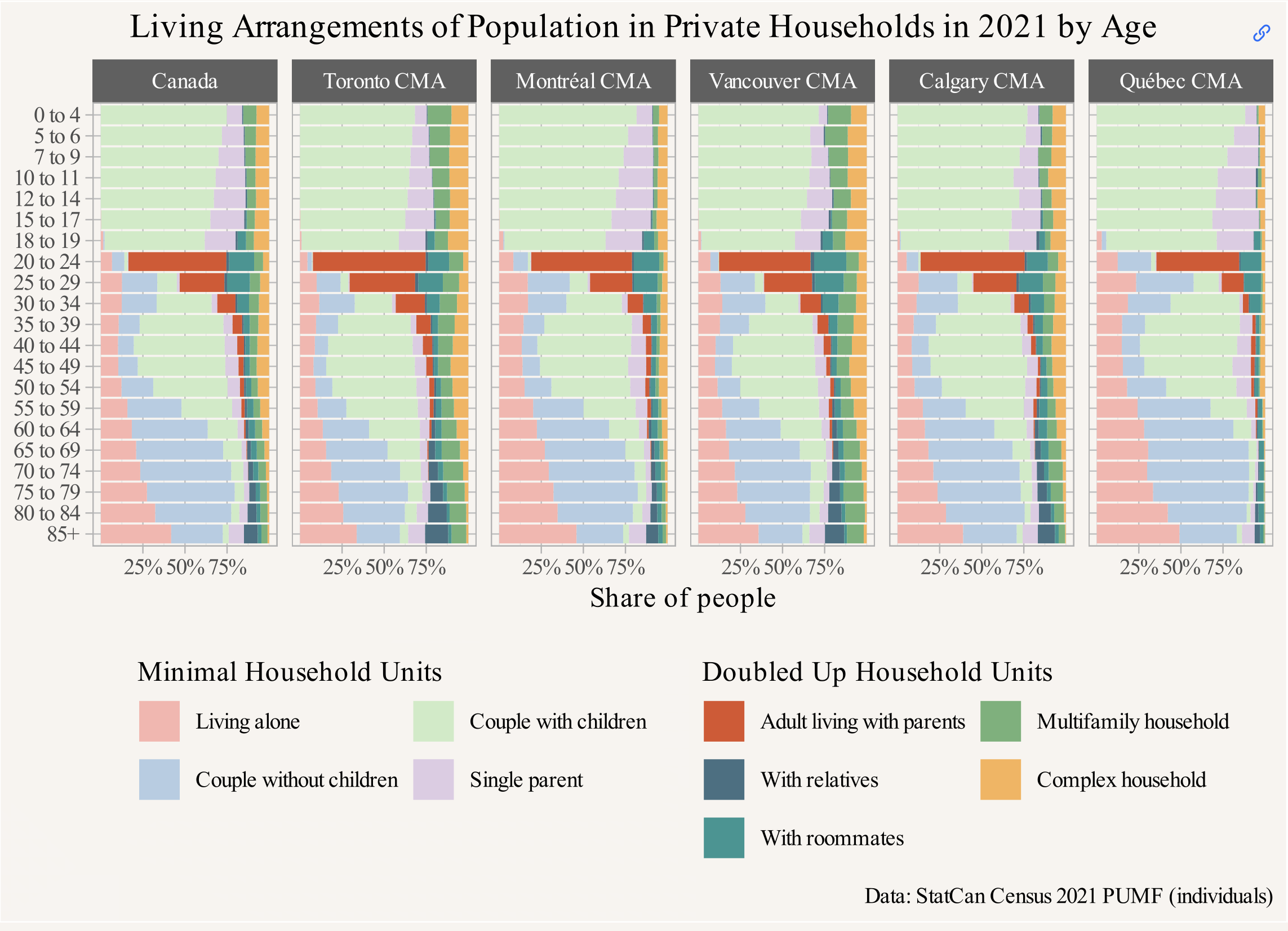
People are, as we keep pointing out, also sloshing around and compressing within containers, where people double up in existing housing when there isn’t enough housing to go around. This is an important mechanism for how housing systems adjust in the short term to demand shocks, but doubling up can also become a long term persistent feature of a housing market. The more people are doubling up all across the metro area, the larger the reservoir of people ready to decompress and fill up new containers wherever they may land, but especially if they land in the most desirable places. Figure 6 shows how people double up by age in Metro Vancouver, and for comparison purposes in select other Canadian metro areas. (Lauster and von Bergmann 2024)
This type of liquidity in housing demographics renders solid demographic models particularly problematic when applied to the sub-metro level, as we explain in more detail below. Where there’s a landscape of desire together with a ready reservoir of demand, we have every reason to expect that where we add new containers will largely determine where people land. Will there still be some empty homes? Sure. But probably not many (von Bergmann and Lauster 2022b), especially when we’ve layered several taxes on to most long-term vacancies. These kinds of taxes can add pressure for sellers and landlords to adjust their prices and rents until people flow into the new containers they control.
In short, don’t count Vancouver out. Short-term sloshing aside, our liquid demography suggests it’s got a decent chance of staying ahead of Surrey. But even in a liquid world, Vancouver may not win! It really depends upon how much housing gets built. Surrey could continue to scale up housing production via more apartments while major investments like SFU’s new medical school could tip the landscape of desire further toward Surrey’s direction. Furthermore, if current policy constraints to more greenfield development, like the Agricultural Land Reserve, come under assault, all bets are off - Surrey’s got a lot more land under ALR protection than the City of Vancouver. But those possibilities aside, in a liquid world there are plenty of reasons to believe that Vancouver will continue to battle off Surrey for the title of most populous municipality in the Metro area. Mostly it just has to keep building more.
City level demographic projections are good in theory, especially if they are done well - ideally by combining our liquid and solid models. But it’s important to understand what they are useful for, and for what purposes they are not well-suited. The solid model pretty much ignores housing. The liquid model strongly emphasizes that in high demand supply-constrained areas, housing determines growth. What we can take away from both is that municipal population projections should not be used for planning around housing needs. Unfortunately, that is exactly what StatCan expects will be done with them:
These projections provide impartial, evidence-based insights to all levels of government, infrastructure owners, operators and investors to improve infrastructure planning and decision-making across Canada. The data is also expected to inform land use and urban planning, housing needs, transportation and communications.
The positioning of the projections as “impartial, evidence-based insights” is a frighteningly naive attempt to cast the assumptions and decisions embedded in the projections as value-free. Treating something that’s mostly liquid and compressible as mostly solid is neither “impartial” nor “evidence-based”. Worse, the notion that projections are expected to “inform land use planning” and “housing needs” is likely to do harm.
Further down StatCan does acknowledge the limitation that “modifications in land zoning” and “local development objectives” can have a big impact on municipal level population growth (“induce rapid fluctuations” in their language). This gets to the key tension: StatCan needs to pick a lane. If local demographics are liquid so land use planning can have significant impact on the projections, then that significantly limits the usefulness of projections that treats local demographics as a solid for land use planning. You can’t have it both ways.
So far we have focused on the M1 projection, StatCan offers a range of population projection scenarios where they vary underlying growth and inter-provincial migration assumptions. This can offer a range of scenarios and planners should not focus on just one of them, but the problem remains that all of these treat local demographics as solids rather than liquids. In Figure 7 we show the full range of scenarios for the City of Vancouver.
van_scenarios <- get_cansim_connection("17-10-0162", refresh="auto") |>
    filter(Gender=="Total - gender",
           `Age group`=="All ages",
           GeoUID=="5915022") |>
    collect_and_normalize(default_month = "01") |>
  left_join(metro_van_cities,by="GeoUID")

rank_data <- get_cansim_connection("17-10-0162", refresh="auto") |>
    filter(Gender=="Total - gender",
           `Age group`=="All ages",
           `Projection scenario`=="Projection scenario M1: medium-growth",
           nchar(GeoUID)==7,
           REF_DATE=="2024") |>
  slice_max(n=10,order_by=VALUE,with_ties = FALSE) |>
  arrange(-VALUE) |>
  collect_and_normalize(default_month = "01") |>
  left_join(metro_van_cities,by="GeoUID") |>
  mutate(n=rank(-val_norm)) |>
  select(GeoUID,Name,val_norm,n) |>
  filter(!is.na(Name))

van_scenarios |>
  filter(Date>="2015-01-01",Date<="2035-01-01") %>%
  mutate(`Projection scenario`=fct_reorder(`Projection scenario`,-val_norm)) |>
  ggplot(aes(x=Date, y=val_norm, color=`Projection scenario`)) +
  geom_line() +
  geom_point(shape=21) +
  scale_linetype_manual(values=line_types) +
  scale_y_continuous(labels=\(x)scales::comma(x,scale=10^-3,suffix="k"),
                     trans="log", breaks=seq(500,900,25)*1000) +
    labs(title="Population Projection Scenarios for the City of Vancouver",
         x=NULL,
         y="Population",
color=NULL) 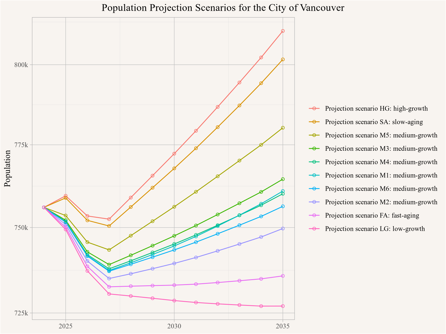
Most of these scenarios are utterly unreasonable. The two highest growth scenarios, the high-growth and slow aging scenarios see Vancouver’s population still increasing in 2025, but then decreasing and only coming up above 2025 levels sometime late 2028.
Of course in the very short term, on the order of a year or maybe two, population could decline. We know there’s sloshing and adjustments that get made even in a liquid world. We’ll get a frozen glimpse at where things stand through the 2026 Census. We have seen such declines before, as during COVID where a multitude of factors came together all at once, as we explained above. But should we really expect one now?
We do know that non-permanent residents consume on average less housing than Canadian born residents, and similarly immigrants consume less housing than those Canadian born (despite what a recent StatCan study claims (von Bergmann and Lauster 2025)). So a reduction in non-permanent residents (and in immigration) may lead to housing being used less intensively, even while people slosh around to fill vacancies. In this sense, we would expect population to go down if the housing stock remained fixed. At the same time, and directly as a consequence of sloshing, we are seeing a softening of the rental market along with a temporary rise in vacancy rate and an increase in properties listed for sale. Altogether these patterns suggest that slightly fewer homes are being lived in until prices adjust to rebalance.
van_stock <- cancensus::get_census("2021", regions=list(CSD="5915022"))$Dwellings

van_current_under_construction <- cmhc::get_cmhc("Scss", series="Under Construction",
                                                 dimension="Dwelling Type",
                                                 breakdown="Historical Time Periods", geo_uid="5915022") |>
  filter(Date=="2025-10-01",`Dwelling Type`=="All") |>
  pull(Value)

van_length_of_construction <- cmhc::get_cmhc("Scss", series="Length of Construction",
                                                 dimension="Dwelling Type",
                                                 breakdown="Historical Time Periods", geo_uid="5915022") |>
  filter(Date=="2025-10-01",`Dwelling Type`=="All") |>
  pull(Value)
But the notion that Vancouver would see sustained population decline while still adding housing is difficult to reconcile with what we know about housing demand in Metro Vancouver. Vancouver has 17,065 units currently under construction alone with an average length of completion of about 21 months, a roughly 5% increase in housing stock that’s already baked in. Will the owners of those units really pay Empty Homes and Speculation and Vacancy Taxes to keep them vacant for long?
We explained how the projections are not particularly useful, but what harm could they do? Mostly the harm comes from when projections are used to justify underbuilding. And this happens a lot.
Turns out that there is a long history of local and regional planning misusing projections like this to restrict housing supply. This is an important part of the story of how we got into our current housing crisis, and Vancouver, city and metro, can serve as a good example.
How does this work? The logic is quite simple. It starts from the assumption that the only reason we need new housing is to accommodate the solid population growth coming out of our assembly line. Then we match the municipal level housing production to fit the projected population growth.
This goes wrong in two ways. First, the assumption that housing is only needed to accommodate population growth (and ageing) is wrong. (von Bergmann and Lauster 2022a, 2025) Things like income growth together with old housing falling into disrepair also increase the demand for housing. Secondly, if projections are mainly based on past trends, as is almost always the case and also true for these StatCan projections, then any past underproduction of housing relative to demand will be baked into the projections. The underproduction of housing becomes self-perpetuating (and gradually worsening) as municipalities use these kinds of projections to plan for future housing.
There is, of course, another way things can go wrong. Planners and politicians can intentionally use their controls over housing to slow population growth.
In the 70s Metro Vancouver regional planning explicitly targeted under-production of housing as a means of managing growth. Growth management became implicitly enshrined using technocratic language within regional growth strategies and housing projection models, which differ in some details but broadly follow the solid demographics that StatCan employed. (von Bergmann and Lauster 2023) The process is quite simple, BC Stats provided local population projections and Metro Vancouver turned them into housing targets for each municipality. For a long time BC Stats considered local community plans for housing to derive the population projections, making this process almost comically circular. Recently BC Stats have changed their method which cuts this circular reasoning, but ironically this has moved BC Stats projections further into the world of solid demographics and made the estimates less suitable (and worse) for the purpose of land use and housing planning. But regional planning authorities seem happy to continue to use them for exactly that purpose.
Similarly, and quite explicitly, a City of Vancouver councillor recently tried to restrict housing production in the city by using exactly these type of arguments and planning processes that, in the face of existing shortages, turn population projections into self-fulfilling prophecies. (von Bergmann and Lauster 2020)
We also have good examples of what happens when population projections turn out to be wrong. Metro Vancouver has been using municipal level population projections for a while and used them to derive housing targets. What can we learn from cases where the projections turned out to be wrong? Quite simply, those were the cases where municipalities did not meet their housing targets. (von Bergmann 2019b) In other words, when there is an existing housing shortage, land use planning drives population growth, not the other way around.
As we noted at the outset, we think people are both liquids and solids. Ultimately we need demographic projections that combine these two forms. But we can go a little further to note that scale matters. At the national level, treating people as solids tends to work out ok. Immigration is subject to controls that really do make people look more like they’re coming off an assembly line. But once people land in Canada, the Charter works to preserve their ability to move freely. As a consequence, people become much more liquid as they move internally. This is mirrored in the reasons people give for moving. Immigrants don’t tend to make the move across borders for reasons like better housing affordability, but within metropolitan areas, housing drives the majority of local moves. Correspondingly, when we get below the metropolitan level, we really need to take into account how people are likely to move in response to where housing is being constructed. In short, at the local level, liquid demographics is the name of the game.
For the race between the City of Vancouver and Surrey that means that it’s mostly up to Vancouver who wins. Demand to live in Vancouver is much higher, if Vancouver allows more housing people will flow toward Vancouver and Surrey will have a very hard time catching up. If Vancouver swings back and cuts down their development pipeline, following Metro guidance, then Surrey will likely overtake Vancouver sometime in the next decade or two. As laid out by Uytae Lee, Surrey seems ready to try.
As usual, the code for this post is available on GitHub for anyone to reproduce or adapt for their own purposes.
## datetime
Sys.time()
[1] "2025-12-08 00:30:33 PST"## repository
git2r::repository()Local: main /Users/jens/R/mountain_doodles
Remote: main @ origin (https://github.com/mountainMath/mountain_doodles.git)
Head: [efd3bd5] 2025-12-08: widgets## Session info
sessionInfo()R version 4.5.2 (2025-10-31)
Platform: aarch64-apple-darwin20
Running under: macOS Tahoe 26.1
Matrix products: default
BLAS: /System/Library/Frameworks/Accelerate.framework/Versions/A/Frameworks/vecLib.framework/Versions/A/libBLAS.dylib
LAPACK: /Library/Frameworks/R.framework/Versions/4.5-arm64/Resources/lib/libRlapack.dylib; LAPACK version 3.12.1
locale:
[1] en_US.UTF-8/en_US.UTF-8/en_US.UTF-8/C/en_US.UTF-8/en_US.UTF-8
time zone: America/Vancouver
tzcode source: internal
attached base packages:
[1] stats graphics grDevices utils datasets methods base
other attached packages:
[1] mountainmathHelpers_0.1.4 sf_1.0-22
[3] dotdensity_0.1.0 rlang_1.1.6
[5] cancensus_0.5.11 cansim_0.4.4
[7] lubridate_1.9.4 forcats_1.0.1
[9] stringr_1.5.2 dplyr_1.1.4
[11] purrr_1.1.0 readr_2.1.5
[13] tidyr_1.3.1 tibble_3.3.0
[15] ggplot2_4.0.0 tidyverse_2.0.0
loaded via a namespace (and not attached):
[1] gtable_0.3.6 xfun_0.53 htmlwidgets_1.6.4 tzdb_0.5.0
[5] vctrs_0.6.5 tools_4.5.2 generics_0.1.4 curl_7.0.0
[9] proxy_0.4-27 fansi_1.0.6 pkgconfig_2.0.3 KernSmooth_2.23-26
[13] tinytable_0.13.0 RColorBrewer_1.1-3 S7_0.2.0 assertthat_0.2.1
[17] lifecycle_1.0.4 git2r_0.36.2 compiler_4.5.2 farver_2.1.2
[21] litedown_0.7 htmltools_0.5.8.1 class_7.3-23 yaml_2.3.10
[25] pillar_1.11.1 classInt_0.4-11 tidyselect_1.2.1 digest_0.6.37
[29] stringi_1.8.7 arrow_21.0.0.1 fastmap_1.2.0 grid_4.5.2
[33] cli_3.6.5 magrittr_2.0.4 e1071_1.7-16 withr_3.0.2
[37] scales_1.4.0 bit64_4.6.0-1 timechange_0.3.0 rmarkdown_2.30
[41] httr_1.4.7 bit_4.6.0 hms_1.1.4 evaluate_1.0.5
[45] knitr_1.50 Rcpp_1.1.0 glue_1.8.0 DBI_1.2.3
[49] rstudioapi_0.17.1 jsonlite_2.0.0 R6_2.6.1 units_1.0-0 This is only counting jobs with a usual place of work people commute to, and estimates from the 2021 census were likely still impacted by the COVID pandemic and proximity to the likely high point of Work From Home.↩︎
@misc{the-trouble-with-municipal-level-population-projections.2025,
  author = {{von Bergmann}, Jens and Lauster, Nathan},
  title = {The Trouble with Municipal-Level Population Projections},
  date = {2025-12-07},
  url = {https://doodles.mountainmath.ca/posts/2025-12-07-the-trouble-with-municipal-level-population-projections/},
  langid = {en}
}