CensusMapper now has 2001 census data, the changes are live and functional and available for mapping and via the data API. We ran some basic verification of the import, and set the metadata for the variables. There may still be some quirks in need of getting ironed out, feedback is appreciated if anyone finds anything that does not look right.
At the same time we finally updated my TongFen package to also include DA level TongFen out of the box, in addition to the CT level that has been working for a while. TongFen is (what we call) the process of making data that originally comes on different geographies comparable, and the TongFen package does that in two ways. It allows for estimates on arbitrary geometries, and it allows re-aggregation of variables from different (Canadian) censuses on a common DA or CT tiling. The latter method does not just result in estimates, but exact counts (up to statistical rounding) at the expense of finding a coarser least common geographic denominator.
This last part is how TongFen got it’s name. Adding fractions involves two steps 1) converting the fractions to the least common denominator and 2) adding the numerators. The first step is hard, even saying it is hard. But in Chinese there is a simple word for that first step: TongFen (通分). Just having a simple word for this process can make it conceptually simpler.
When working with geospatial data on different (but somehow comparable) geometries we face essentially the same challenge: finding the “least common geography”. The TongFen package is makes that step simple by completely automating it. From finding the least common geography to aggregating up the variables, paying attention to if the census variable is e.g. a simple count or a percentage or maybe the average income and aggregating the values appropriately and autonomously.
So let’s see how this works by comparing 2001 and 2006 dwelling data. With the purpose of the post being to showcase the new data and methods as much as to shed some more light onto how census methods effect how the census sees dwellings, we keep most of the code visible on the main page for this post.
Dwelling type data
Let’s see how this works by exploring some of the changes in census methodology between the 2001 and 2006 census that has tripped up people in the past. The census changed the way it counts dwelling units, in particular it started hunting around for secondary suites.
Using the cancensus and TongFen that’s easy. We first search for the variables on “structural type of dwelling” and grab all the child variables. Then we grab the data for the City of Vancouver on a common 2001 and 2006 geography using the TongFen package.
vectors_01 <- search_census_vectors("structural type","CA01") %>% rbind(child_census_vectors(.))
vectors_06 <- search_census_vectors("structural type","CA06") %>% rbind(child_census_vectors(.))
all_vectors <- c(vectors_01$vector,vectors_06$vector)
regions <- search_census_regions("^Vancouver$","CA01") %>%
  filter(level=="CSD") %>% as_census_region_list()

data_da <- get_tongfen_census_da(regions=regions,vectors = all_vectors,geo_format = 'sf')
With the data at hand we compute the change in single detached and duplex dwellings, and discretise them for mapping purposes.
change_breaks <- c(-Inf,-100,-50,-25,-10,10,25,50,100,Inf)
change_labels <- c("Lost over 100","Lost 50 to 100","Lost 25 to 50","Lost 10 to 25","About the same",
                   "Gained 10 to 25","Gained 25 to 50","Gained 50 to 100","Gained over 100")

plot_data <- data_da %>%
  mutate(duplex_change=v_CA06_123-v_CA01_116,
         sd_change=v_CA06_120-v_CA01_113,
         dwelling_change=Dwellings_CA06-Dwellings_CA01,
         household_change=Households_CA06-Households_CA01,
         unoccupied_change=dwelling_change-household_change,
         unoccupied_01=Dwellings_CA01-Households_CA01,
         unoccupied_06=Dwellings_CA06-Households_CA06) %>%
  mutate(sd_change_d=cut(sd_change,breaks=change_breaks,labels=change_labels),
         duplex_change_d=cut(duplex_change,breaks=change_breaks,labels=change_labels),
         unoccupied_change_d=cut(unoccupied_change,breaks=change_breaks,labels=change_labels))
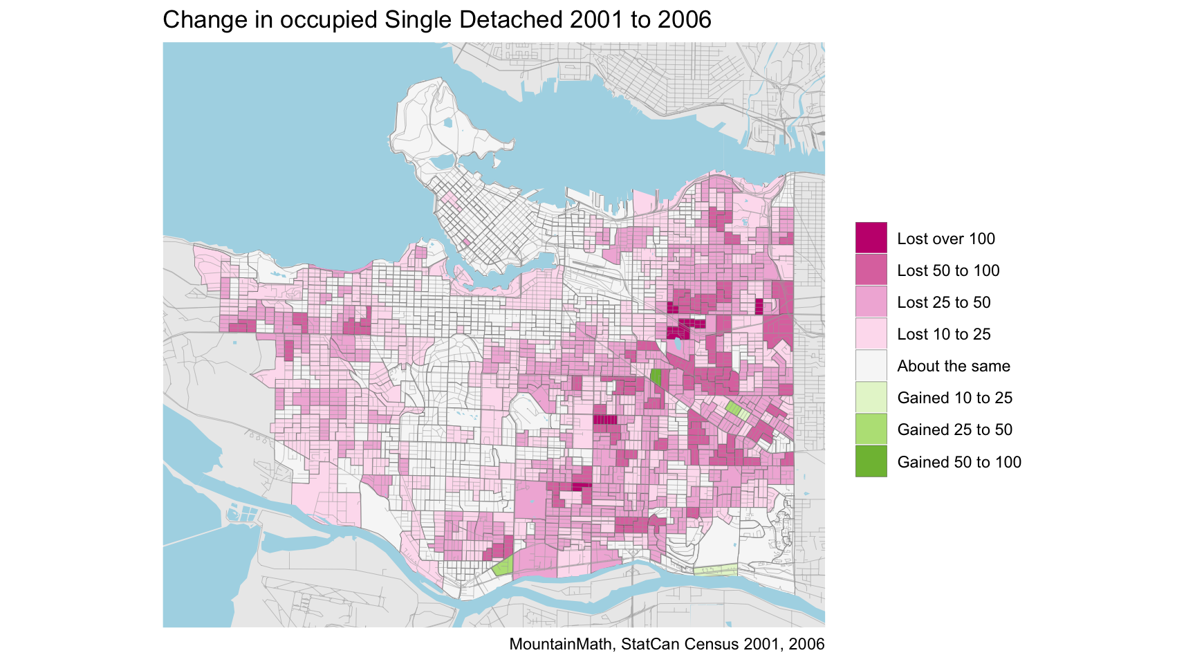
Overall StatCan reports that Vancouver lost quite a few single detached dwellings between these censuses, 17,045 in total (net) to be precise. Let’s map them to understand the geographic distribution of the lost single detached dwellings.
ggplot(plot_data) +
  geom_sf(aes(fill=sd_change_d),size=0.1) +
  change_map_theme +
  labs(title="Change in occupied Single Detached 2001 to 2006")
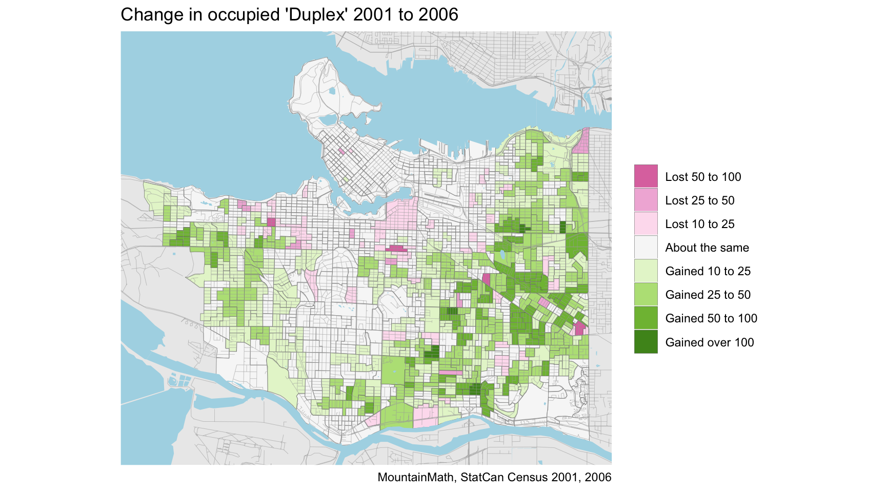
The bulk seems to be in Vancouver “single family” neighbourhoods, so what happened to them? The answer to that is simple, in 2006 the census started hunting for secondary suites. And a single detached house with a secondary suite is not “single” detached any more, but classified as a “duplex” in census language. Mapping the change in duplex units reveals that there is a reasonably good match.
ggplot(plot_data,aes(fill=duplex_change_d)) +
  geom_sf(size=0.1) +
  change_map_theme +
  labs(title="Change in occupied 'Duplex' 2001 to 2006")
Except it’s never quite that simple. For every single detached home where the census found a secondary suite, the census now counts two units instead of one. Eyeballing the map it does indeed seem like there may be more duplex units gained than single detached lost, but are there really twice as many?
That question comes down to two details: 1) The modifier in the map title that we have not yet talked about: We are only looking at occupied units, not all units. The best way to resolve this is to get a custom tabulation to look at structural type of dwellings for all dwelling units, not just the occupied ones. We have done that using 2011 data and found that secondary suites are the most likely type of dwelling to register as not occupied (by usual residents). 2) “Apartments, fewer than five storeys”. This is the census classification for anything with fewer than five storeys and more than two units. Including for a “single family” home with two secondary suites. If the census found homes with single secondary suites (“duplex”) it will also have found homes with two secondary suites.
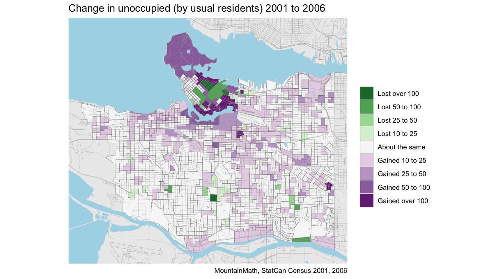
But that’s for another time to untangle. To close this off let’s look at the overall change in units not occupied by usual residents.
ggplot(plot_data,aes(fill=unoccupied_change_d)) +
  geom_sf(size=0.1) +
  scale_fill_brewer(palette = "PRGn",direction = -1) +
  map_theme +
  labs(title="Change in unoccupied (by usual residents) 2001 to 2006")
We do see a general increase in those units in the areas that saw single detached get reclassified into duplexes, but what stands out is the activity near new developments. Both areas where buildings were completed just before the 2001 census and that filled in by the 2006 census, as well as near buildings that completed close to the 2006 census date and have not filled in yet.
Unfortunately we don’t have this data at the census block level, which makes it easier to identify single buildings that drive the change in unoccupancy numbers.
Summary
With 2001 data now available we get longer timelines to understand how our cities change. And the added ability for DA level comparisons in the TongFen package make it super-easy to analyse change on fine geographies. A general caveat here is that at DA level statistical rounding plays a role, as well as other issues with census data including geocoding problems.
As usual, the code for the post is available on GitHub for those interested in replicating or adapt this for their own purposes.
Reuse
Citation
@misc{2001-census-data-and-tongfen.2019,
  author = {{von Bergmann}, Jens},
  title = {2001 {Census} {Data} (and {TongFen)}},
  date = {2019-06-03},
  url = {https://doodles.mountainmath.ca/posts/2019-06-03-2001-census-data-and-tongfen/},
  langid = {en}
}
