How not to analyze the roots of the affordability crisis

Another “working paper” on Vancouver’s real estate woes came out, this one by Josh Gordon. We have been contemplating for a week now if it is worth responding to, but after seeing one too many obviously false statements about what the working paper supposedly shows making the rounds, we felt the benefits of addressing this might outweigh the costs of further entrenching the camps in Vancouver’s real estate debates with this post.

For those that don’t have the patience to read the whole post, feel free to jump around between the following fairly self-contained sections.

• The affordability measure used (spoiler, it’s pretty terrible unless you live in a fantasy world)
• The numbers going into the affordability measure (spoiler, they are wrong)
• Mismatch of metrics (and why the mismatch is a problem)
• The real world (real world data gives different results)
• The ecological fallacy (technical, but important problem for causal inferences)
• How to fix this (some overview and link pointing to how to do this better)
• Addendum (addressing some of Josh Gordon’s comments on a pre-version encompassing the post up to this section)

Affordability measure

The author measures “affordability” using the price to income ratio, defined as “average [detached] house price to average household income”, taken at the municipal aggregation level. This is a curious choice of metric. Why average household incomes? Why include renters in the income metric? Why single family homes and exclude other types of homes? Why aggregate at the municipal level before taking the ratios? We are left to guess, but the underlying assumption that would justify this metric is that every households should be able to buy a single-detached home in the municipality they currently live in. Unfortunately that only makes sense in some fantasy universe, but it does make for catchy price to income ratios.

The numbers

In Figure 1 of the working paper we are shown how this supposedly played out in 2016. Household income is a concept that’s only available in the census, so the graph likely made some adjustments to extrapolate from the average household income reported in 2015 to 2016. One way to do this is to scale the 2015 incomes by the Metro Vancouver growth in median family income of 2.85% between 2015 and 2016. While not a perfect substitute, this should give a reasonably good measure.

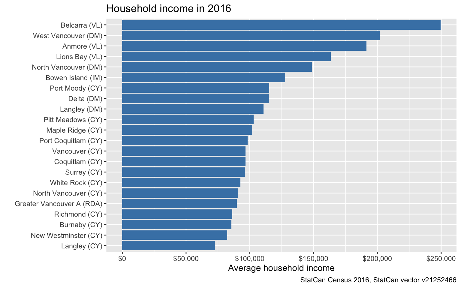
It’s immediately apparent that these numbers differ dramatically from those in the working paper. Looking at West Vancouver the working paper underestimates the average household income by almost a factor two, and that’s still not counting some sources of income like capital gains income, which averaged $27k per household in 2010. (We don’t have 2015 numbers handy.) Or RRSP withdrawals which likely are above average in communities like West Vancouver, which has the highest share of seniors in Metro Vancouver at 28% of the population. For some other municipalities, for example Maple ridge, the average household income estimate in the working paper still comes out short, but only by less than 10%.

In case this needs saying explicitly, any analysis that’s based on comparing metrics based on such wildly incorrect income numbers is bound to produce wrong results..

There probably are some income numbers of some type that match those used in the analysis, and the income numbers are defined and labelled incorrectly throughout the text. Who knows, either way the metric is constructed extremely carelessly. But the main issues is actually not that the input metrics of the analysis are grotesquely off, that part is reasonably easy to fix by just substituting in better estimates. The main issue is that the methods of the type of analysis performed with the metric is flawed, as we will explain in the following sections.

Mismatch of metrics

The main metric employed in the working paper suffers from a severe mismatch of populations the aggregate is taken over, as we already noted above. The income metric is taken over all households, whereas the price metric is taken over all detached dwellings (as defined by the real estate boards). These two metrics match up in the case of an owner-occupied detached dwelling, while mismatches occurs for non-owner occupied detached dwellings on the dwelling side, and renter households as well as owner households in attached dwellings. This makes the price to income ratio as defined in the working paper very hard to interpret, we have written about this problem before.

To appreciate the effect of this mismatch, we can look at the average income of owner households in single detached housing (where some smaller municipalities are aggregated into groups) using a custom tabulation we have worked with before.

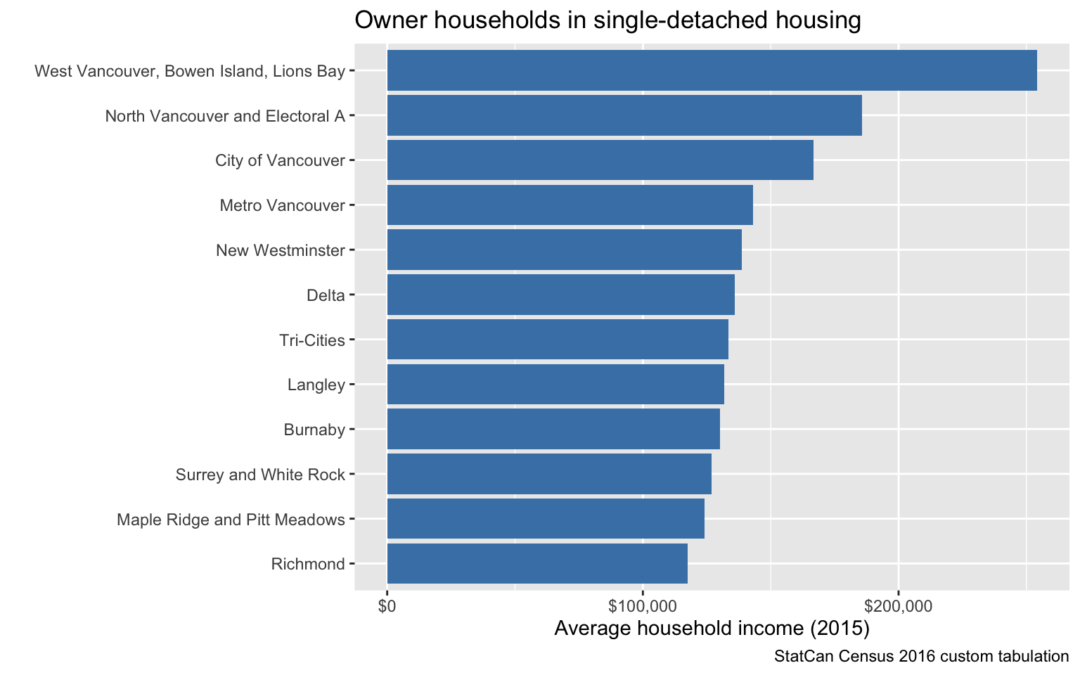
As expected, the numbers come out significantly higher than overall household incomes, but the respective ranking is also different. When just looking at owner households in single detached housing, such households in for example the City of Vancouver have higher income than those in Delta, but overall average household income is higher in Delta than in the City of Vancouver.

The reason for this is of course that detached homeowners come from a different portion of the income distribution in different municipalities, a textbook example of the Simpson’s Paradox that the working paper falls prey to. There are several other income metrics one may want to choose, for example one can exclude senior households, or external migrants within the previous year where income numbers are uninterpretable. Or use medians instead of averages, or use adjusted family income, or work with the full income distribution. Any of these choices will lead to different overall numbers, as well as differences in the ranking.

The bottom line for the working paper is that the correlations at the aggregate level are quite sensitive to the choice of input metric. In particular, the metric chosen in the working paper, is prone to lead to analysis skewed by household composition, with e.g. 38% of households in the City of Vancouver being 1 person households, which tend to have significantly lower incomes than family households, compared to 20% in Delta. On the dwelling side, in the City of Vancouver roughly 28% of dwelling units are detached, compared to 72% in Delta. Looking at tenure, 46% of households in the City of Vancouver are owner households, compared to 78% in Delta. These differences alone explain a good portion of why the rank of the two municipalities switches depending on the choice of income metric. And they illustrate how the analysis in the working paper is heavily confounded by the differing demographic composition of the municipalities.

It is very unfortunate that the report completely ignores these issues, with the exception of the case where the report argues to remove an the City of Toronto as an “outlier” because “pooling many lower income renters (who typically live in apartments) with higher income detached homeowners [has the effect of] boosting the price to income ratio”, and because of “relative rarity of detached houses” with “rezoning potential” – arguments which all apply to the City of Vancouver to a higher degree. Unfortunately, these kind of selectively applied case-by-case arguments are endemic in the report, underlining the complete lack of methodological framework.

The real world

So how about those correlations between incomes and home prices? Josh Gordon writes

[W]e should see a strong positive correlation between housing prices and household incomes by sub-area in an urban region. Yet in Vancouver, the correlation was virtually non-existent.

His analysis shows that that statement is true in Josh Gordon’s fantasy world where average household income numbers are vastly different from reality, and where every household should be able to buy a single family home in the municipality they currently live in.

Meanwhile, let’s check how things play out in the real world, where people live in different kinds of housing and different tenures, we can compare incomes and home values of owners living in their homes. We can do that for all owner-occupiers, or just for owner-occupiers of single detached homes. Or for those in apartment condominiums.

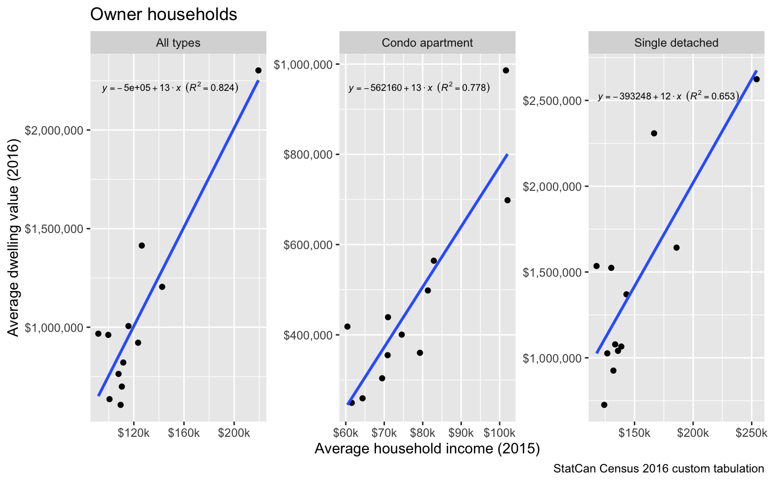
And indeed, we see a strong positive correlation between average households incomes and average home values of owner-occupiers in our 12 regions. The average dwelling values here are based on self-estimated values, which will likely have some variance for individual households, but in aggregate are fairly close to average sale prices around that time. Just to check this, we give a labelled graph of the average dwelling values.

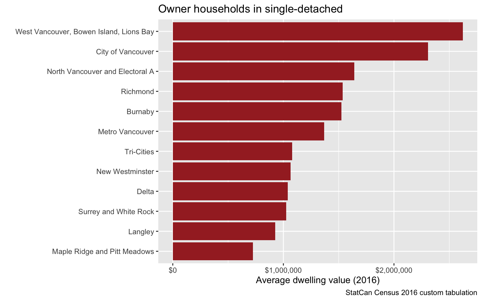
The dwelling values come out close to the values used in the working paper, accounting for the grouping of municipalities in our dataset.

We can also check the price-to-income ratios.

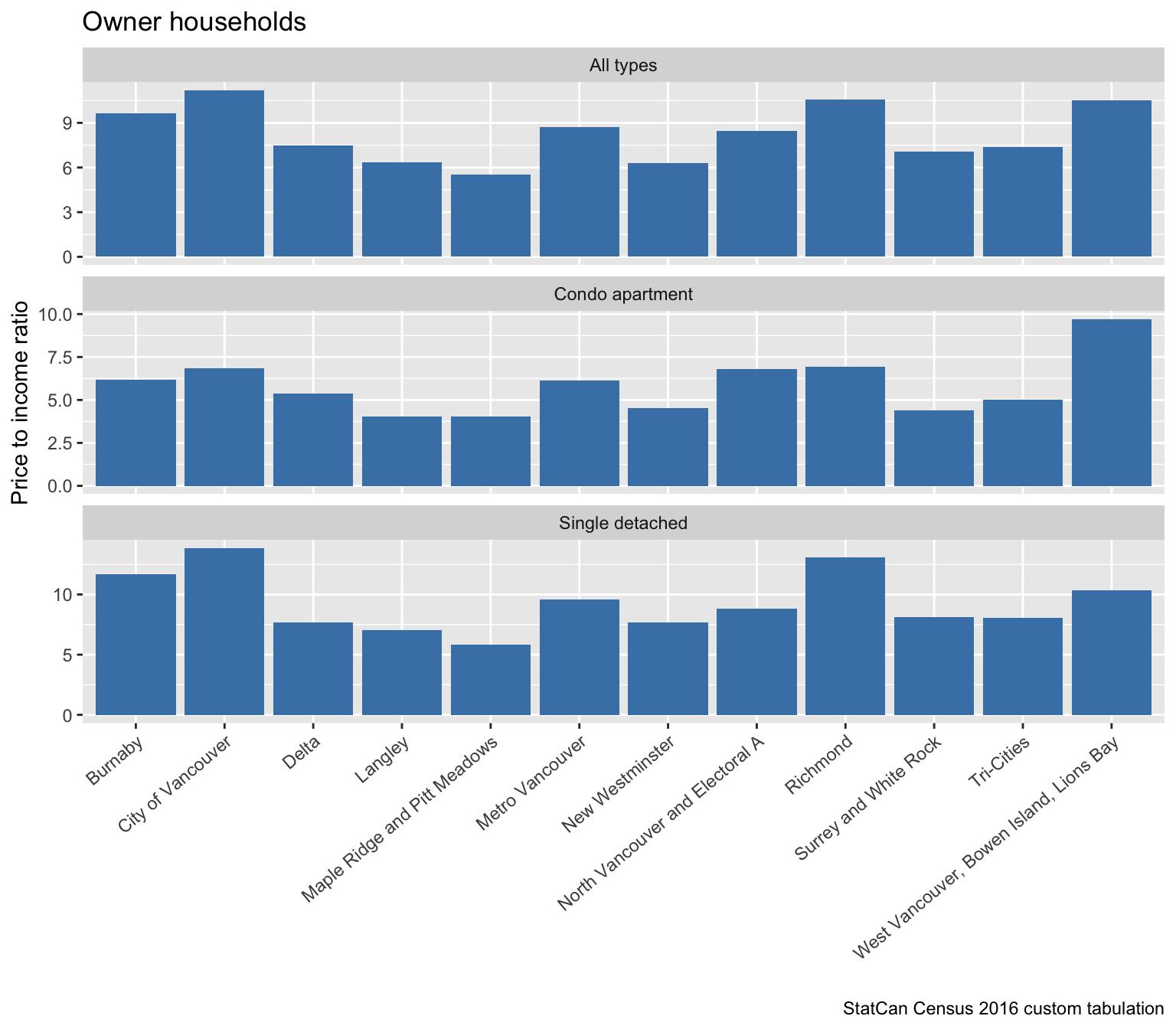
Those are very high price to income ratios, but nowhere near the ones the paper reports for the fantasy universe. As noted in the working paper, wealth likely plays a significant role for people purchasing homes, as will Canadian income sources not accounted for in Census income numbers we already mentioned above, as well as gifts, inheritance, and also unreported income earned abroad.

Ecological fallacy

The report proceeds to introduce a second metric, the share of non-resident owners in each municipality and correlates them with the price to income metric. The obvious issues arising from the mismatch between CHSP’s “single detached” and the real estate board’s “detached” categories go completely unmentioned.

The report then attributes the strong correlation these metrics exhibit to the buying behaviour of non-resident owners, which is a textbook example of the ecological fallacy. The report takes no steps to mitigate this despite this fallacy being well-known for often producing wrong results to the degree that it can even reverse the sign of correlations run on ecological vs individual level data. In short, the conclusions drawn from the correlational analysis in the working paper are well-known to be highly problematic, in particular this renders the paper’s attempts to establish causation to nothing but wishful thinking in the hopes that the ecological fallacy does not apply. Let alone that the other variable in the correlation, the price to income metric, is incorrectly calculated and has little meaning outside of the author’s fantasy universe of single family abundance.

To round this off we quickly check how the ecological correlations with non-resident single-detached owners play out in the real world.

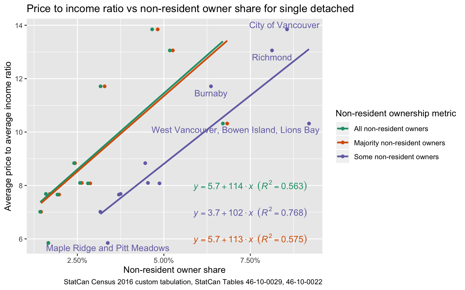
This gives still a reasonably strong correlation, although with a much lower R² that depends to a significant degree on the choice of non-resident owner metric chosen. In particular this shows that the lazy argument in the working paper asserting that the choice does not make a difference is not correct. And this is not a product of our grouping, correlating the grouped majority vs any non-resident participation gives an R² of 0.947, not much different from the 0.959 in the ungrouped data.

While we have reduced some of the unaccounted confounders by moving the price-to-income ratios from the fantasy world to the real world, it would be foolish to assume that this was the only confounder at play, let alone not having dealt with the ecological inference problem. The regions with large residuals give an indication of missing confounders, with the commute distance to the central business district being a strong contender in fitting the general model of how people make trade-offs between housing and transportation costs.

How to fix this?

Increasing the overlap between the populations for the price and the income metric is a simple starting point, and above we have outlined how that plays out in the real world. Increasing the geographic granularity is another, municipalities is too coarse a geography with very high demographic variability to be useful for aggregate metrics in this kind of analysis. We did both in a report back in 2016. But this only reduces issues around Simpson’s paradox, it does not completely remove them. And this path still bumps into the ecological fallacy if one wants to use this to attribute variations in the price to income ratio to behaviour of individuals within those regions, and thus can’t provide much insight into causation. There are ways to mitigate this problem, but for the particular argument made in the working paper the metric on share of non-resident owners is only available at the municipal level. This does not give enough regions to have much hope in removing the underlying issue, the aggregate metrics simply don’t carry enough information for such inferences.

A much better and more straight-forward route is to take individual level price to income ratios, and analyse how these vary across a variety of other parameters. Care needs to be taken to do this properly, we have some examples of how one could do this. On a descriptive level, we can simply check who lives in high-value homes that the report is so focused on. We have done a descriptive analysis detailing several variables of owner-occupiers of high-value homes, including price-to-income ratios. One can take this further and add more variables to understand owner households in very high price to income situations, along the lines Nathan Lauster and I have done to understand households that might get caught in speculation tax audit triggers based on price to inocome ratios as well as for how long they have lived in the home. For this we used PUMF data, which provides great flexibility to explore and fine-tune metrics at the expense of higher uncertainty and coarse geographies, but this can of course be remedied by pulling a custom tabulation once one has a good understanding of the metrics and variables one is interested in. This approach has the added advantage of allowing to loosely separate out recent buyers.

One disadvantage of this approach is that it does not give information on buyers that don’t owner-occupy their place. At this point, the only thing we know about these places is if the owner lives in Canada or overseas using CHSP data, or if the place is rented or vacant using census data. But we can’t even crosstab these metrics although CHSP is working on developing measures of how the non owner-occupied homes are used.

The upshot

Taking a step back, the working paper tried to offer insight into what drove the housing market in Vancouver (and Toronto). I am looking forward to reading work that will add insight to this question, using rigorous methodology. I am afraid Josh Gordon’s working paper does not do this.

It should also be pointed out that this post should not be read as an analysis in it’s own right. In particular, the scatter plots presented still contain numerous unaccounted confounding factors. This post is not aimed at offering an alternative analysis, but it simply serves to illustrate the methodological failings in Josh Gordon’s working paper. For insight into mismatches between housing and income metrics we refer the reader to the posts linked in the previous section that build on individual level price-to-income and shelter-cost-to-income metrics.

As usual, the code for the analysis is available on GitHub in case someone wants to check the details, or adapt the analysis for their own purposes.

Addendum

I sent this post to Josh Gordon before distributing it, and he had a couple of comments he asked I address in my post.

Firstly, he asserts that he has been using median household income numbers throughout, despite claiming he used average household income in his paper. We already establish above that the paper did not use average household income numbers, and the numbers don’t match median household income either, adjusted for 2016 or otherwise, as a quick comparison shows. We still don’t know what income statistic was actually used in the paper.

Secondly, Josh reiterates that one should use income numbers for the whole population as opposed to matching home prices to the incomes of the population that lives in those homes as I suggested above, because “non-owners are in many cases potential owners and so their incomes matter in terms of what your housing market should look like if it’s connected to local incomes”. Josh further submits that

There’s also a utility to simply understanding whether a typical resident can afford a typical detached home, and so eliminating much of the bottom half of the distribution is going to give you a flawed understanding of that. Certainly for most renters in Vancouver, the fact that detached houses, which most would ideally like to reside in, are sometimes between 20 and 30 times their income is relevant and part of the affordability issues Vancouver faces.

While I appreciate the plight of renters looking to buy a home (some of which may be looking to buy a detached house) and agree that there is utility in understanding how these people fare, this simply isn’t what Josh is constructing his metric for. And I am baffled by the consistency with which Josh ignores the simple geometric fact that the City of Vancouver’s ~75k detached homes aren’t able to house Vancouver’s over 280k households, and that given that “most would ideally like to reside in” one of these one should expect the median price of these homes to be governed roughly by people in the 90th percentile of the City of Vancouver income distribution, assuming that home prices are aligned with incomes. So if one wants to test this alignment (or lack thereof), one needs to consider the household at the 90th income percentile. Using the 50th percentile, as Josh keeps insisting, is simply not informative but serves to collect confounders, as the share of detached homes and the shape of the income distribution varies across municipalities. But we already explained this at length above.

Josh states that I should not include Anmore and Belcarra in my analysis because there too few detached houses there, but apparently he fails to notice that I grouped them together with nearby municipalities. To do this properly would require setting up a methodological framework that properly deals, among other things, with different municipalities having different numbers of dwellings and households. This could be as simple as using weighted regressions, but given how few data points are being used the analysis would likely benefit from a more sophisticated statistical model, which would also guard against the post-hoc nature with which the report attempts to discard “outliers”.

Next Josh makes the point that my use of average price to income ratio might get skewed by outliers. My choice was of course triggered by what he claimed he used, but this is still a valid concern and again points to individual (as opposed to aggregate) level price-to-income being the more useful metric. And he asks that I redo my analysis based on his “standard methodological decisions”, and says he will “simply screenshot this email exchange and it will be posted under [my] blog post on twitter” if I fail to do so. Which, quite frankly, is not just incredibly rude, but also impossible because Josh has not actually made his methodology clear. One would first need answers to the following questions:

• What income metric is being used and why?

• What price metrics are being used and why? (Josh asserts he is using REBGV benchmark prices, which is clearly false as REBGV does not cover some of the Metro Vancouver municipalities reported on in the working paper.)

• Why can we assume confounding factors, including the ones I outlined above, are not skewing the results?

• Why can we assume the ecological fallacy won’t affect the results?

• Why was the particular non-resident owner metric chosen, as opposed to e.g. using majority of owners living abroad, or all owners living abroad. (The argument Josh makes that it does not matter because they all correlate is incredibly naive and incorrect, as shown in the main part of this post.) And what exactly is the non-resident owner metric is being used as a proxy for? (Josh asserts it’s “ownership primarily based on foreign income or wealth”, which is an frustratingly ill-defined concept.)

• Is the working paper actually claiming to show causation, and if yes, how?

These are, quite frankly, pretty standard methodological checkboxes for scholarly research, which the working paper is being presented as. And I am happy to revisit this and take a fresh look at the “methodological decisions” once the paper actually lays them out properly. As it is, Josh’s paper is a mess. And I don’t feel it’s my job to clean it up.