Geographic data often comes on different geographic breakdowns. A prime example is census data, where the underlying census geographies can change from census year to census year. This makes it difficult to compare census data across censuses. But comparing census data across censuses at fine geographies is important for many applications.
There are two main ways how people deal with this problem. 1. Estimate data for one of the two geographies by (usually at some point) relying on area-weighted interpolation. 2. Aggregate up areas in both geographic datasets until one arrives at a common tiling.
The first method has the advantage that it always works, but the disadvantage that it is only an estimate and inevitably produces incorrect estimates. One example of an effort along this lines is this dataset giving weights to pairs of Canadian census tracts across the 1971 through 2016 censuses, details can be found in this article. Analysis based on this method needs to include an extra level of sensitivity checks to quantify how sensitive the analysis is to the assumptions (implicitly) used in the estimates. I am not aware of a good tool to aid such a sensitivity analysis, which significantly diminished the usefulness of this approach for academic research.
The second method has the advantage that it’s (fairly) exact. The Statisitcs Canada Correspondence files are a prime example of this approach, they encode instructions on how to link geographies in each census in order to achieve a common tiling. While only correspondence files for adjacent censuses are available, and the only geographies covered are Dissemination Blocks and Dissemination Ares, this can be trivially extended to span multiple censuses and other census geographies via joining multiple tables.
TongFen
Both of these methods have value, and we have incorporated them into our TongFen, which has become an integral part of our data analysis pipeline.
The tongfen_estimate function provides the ability to estimate data given on one geography on a different geography. It is essentially a downsampling method that distributes data from a larger geography into smaller geographies. In its simplest form this reduces to area weighted interpolation, and can be extended to dasymetric interpolation via the proportional_reaggregate function if other contextual data, for example Dissemination Block level counts in the census context, or secondary data like land use patterns that can help reduce downsampling errors, are available. It handles arbitrary geographies and is not constrained to any particular type like e.g. census tracts.
This is the method we use when geographies aren’t congruent in the sense that they don’t support a common tiling (other than aggregating the data into a single unit), or when we have fixed geographic target areas that we don’t want to aggregate up further. A rundown of how to use this method, including refining via dasymetric estimates, as well as an analysis in the errors this introduces, can be found in our example estimtes of census data for Toronto Wards, where a custom tabulation with exact counts is available as an authoritative check against the estimated values.
Because of the implicit and hard to estimate errors when estimating data for a fixed target geography we try to resort to aggregating areas up to a common tiling whenever possible. This process, making data comparable by finding a (least) common geography, is what we call TongFen, named after the Mandarin word for bringing two fractions onto the same (lowest) common denominator.
We have demonstrated this using multi-year census data for Vancouver and for Toronto and more recently using Census Tract level annual CRA tax data (https://doodles.mountainmath.ca/blog/2020/04/23/census-tract-level-t1ff-tax-data/), and this is also what’s baked into CensusMapper for 2011/2016 comparative interactive maps. The main drawback is that StatCan correspondence files are only available for census geographies, and that they only allow linking of census data back to 2001. On the plus side, the TongFen package leverages CensusMapper metadata to also automatically aggregate up the census variables, which can be a bit of a headache when dealing with variables that aren’t straight-up counts like averages or percentages. But this breaks down for medians, medians can’t be aggregated up this way and TongFen resorts to estimation instead (while emitting a warning message).
Universal TongFen
There are two obvious ways to extend the existing methods. One is to add tools for automated sensitivity analysis to accompany tongfen_estimate, which is still work in progress. The other is to extend TongFen methods that aggregate geographies to a common tiling for arbitrary geographies, not just the ones where we already have correspondence files like the 2001 through 2016 censuses. That’s what we mean by universal TongFen. At the base of this the new estimate_tongfen_correspondence function that generates a correspondence between two arbitrary geographic datasets. We will first demonstrate how this works using census data, and then apply this to federal election polling district level data.
Estimating correspondence files
To start out we need to understand why this necessarily is a matter of estimation and not computation. Geographic data tends to be messy and the spatial accuracy of geographic dataset varies. Because of the nature of how inaccuracies enter into spacial data, these accuracy issues tend to be distance based.
When finding a common tiling of two separate geographic datasets we have to answer the question when we consider geographic regions form each of the datasets to be “the same”. The estimate_tongfen_correspondence function addresses this by allowing the specification of a tolerance parameter, that determines by how much we allow regions to differ before we consider them to be different regions.
To see how this works let’s take a look at the dissemination areas in the City of Vancouver, including Musqueam 2 and the unincorporated area around UBC to the west.
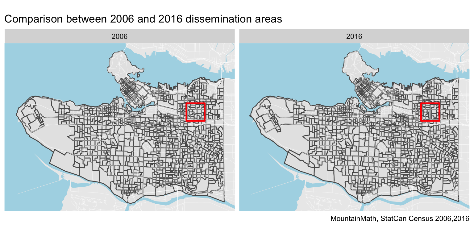
Most of the areas appear unchanged between the censuses. We notice some larger changes highlighted in the red square, let’s take a closer look.
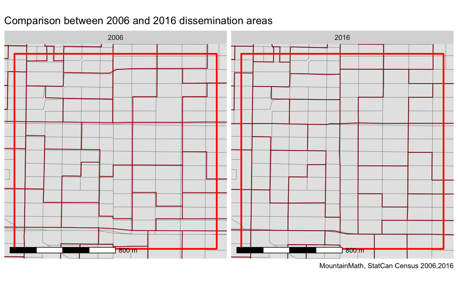
Zooming in, and using the fixed road network (taken from Open Street Map) for reference, we notice that next to the larger boundary changes where polygons got re-assembled, many of the other polygon boundaries changed slightly between 2006 and 2016, mostly to better align with the road network.
This gives us some indication of what kind of tolerance we want to choose when trying to match up the areas. A 10 metre tolerance will probably trip up on some of the small boundary adjustments to better align with the road network, but if we choose the tolerance too large we might miss meaningful boundary changes. Given that a typical lot in Vancouver is about 110 feet deep, a 30 or 40 metre tolerance will be probably coarse enough to allow for minor alignment adjustments, but fine enough to pick up boundary changes that move one lot to a different geographic area.
We can put that theory to the test by plotting the results of estimate_tongfen_correspondence with 10, 20, and 30 metre tolerance, while also plotting the original geographies and the results of using get_tongfen_census_da that utilizes the official StatCan correspondence file for matching up regions.
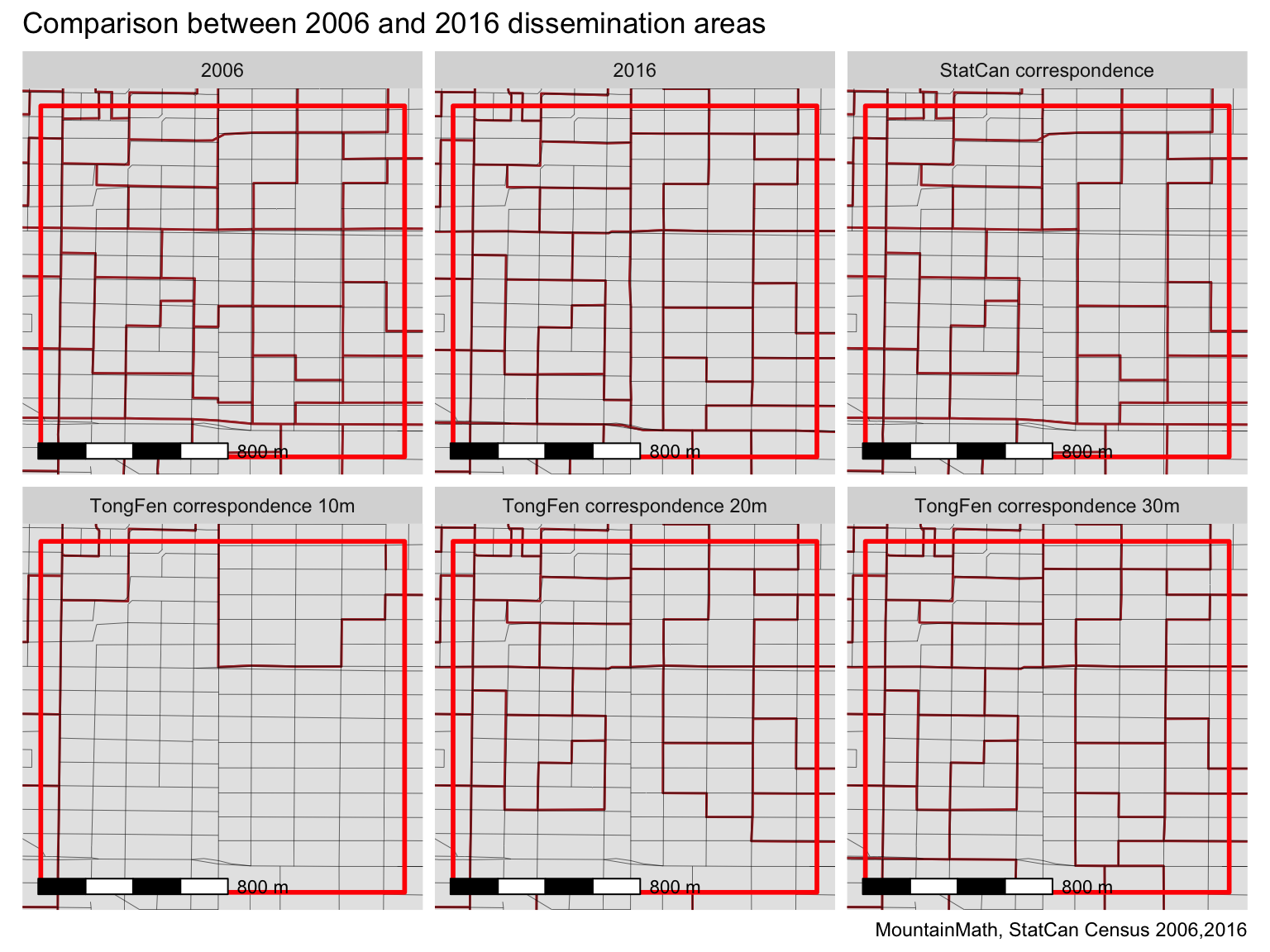
Indeed, using 10 metre tolerance gets tripped up on a lot of the minor boundary adjustments and amalgamates the geographies into large regions. A 20 metre tolerance gets a much finer view, but still get tripped up by the boundary adjustments along Broadway along the bottom of our area of interest. The 30 metre tolerance seems to strike the right balance, at least of the geographies in this map view.
We notice a difference between the amalgamation using the StatCan correspondence files and the 30 metre tolerance estimate in the top right quadrant, where the StatCan correspondence files tell us to dissolve an east-west boundary that our estimate_tongfen_correspondence leaves untouched. This is likely a change introduced by StatCan because of issues of comparability for the data across those censuses, possibly due to geocoding errors across the boundaries. In theory it could also be due to boundary changes in the 2011 census, as the StatCan correspondence files between 2006 and 2016 are bridged by the 2011 geographies, but closer inspection reveals this is not the culprit in this case.
For completeness here is a comparison of the 2006, 2016, TongFen based on the StatCan correspondence files and TongFen based on estimating the correspondence via estimate_tongfen_correspondence. Next to our 30m tolerance, we’ll throw in estimates based on 50m and 100m tolerance.
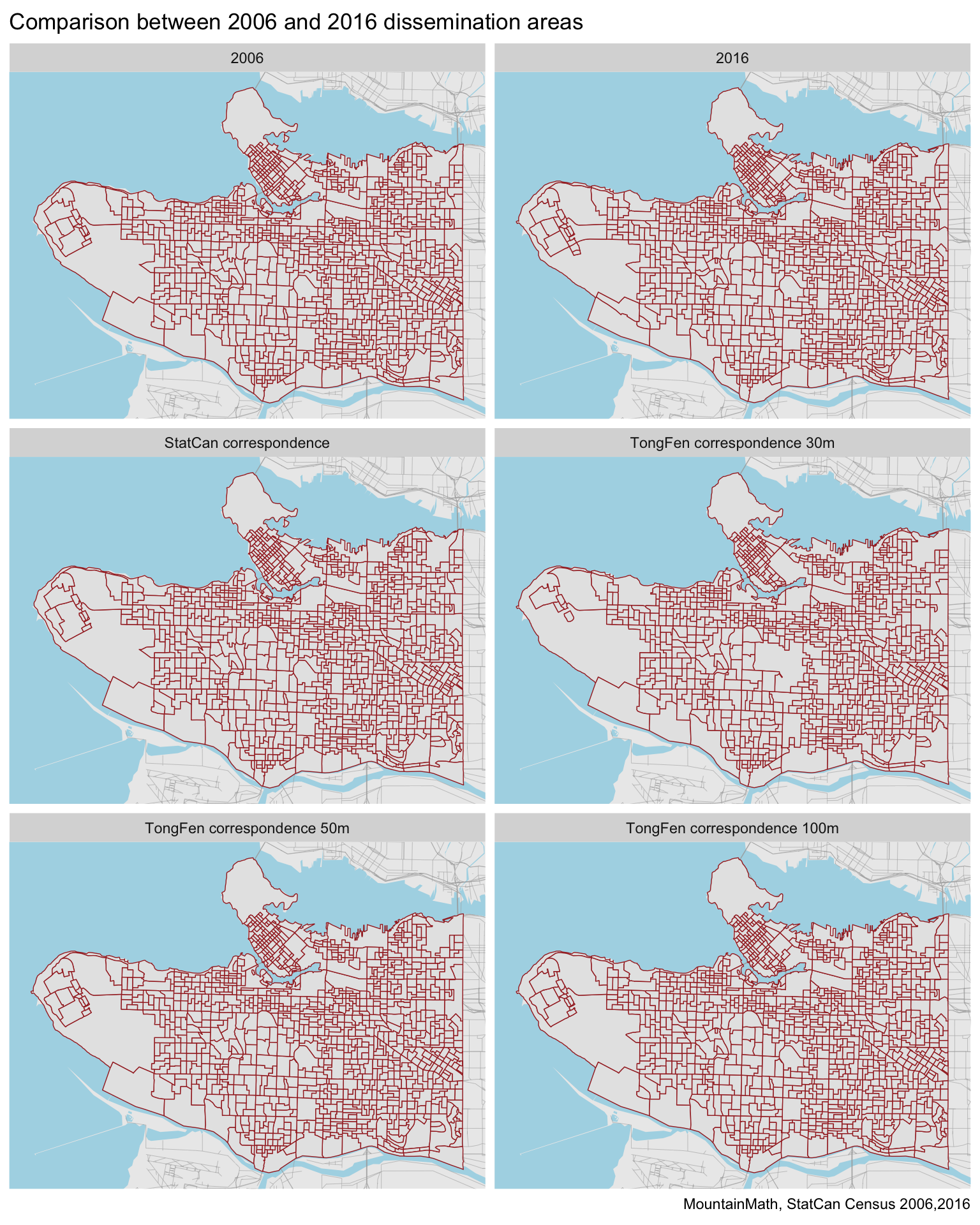
The TongFen estimates with 30 metres tolerance still loose a fair bit of detail in several areas, especially where census boundaries are curvy and 2006 tracing of them is proving rather rough.
The 50m tolerance recaptures a lot of the lost detail, but also fails to amalgamate some ares where the StatCan correspondence files dictate a boundary change should have happened, for example at UBC. However, the StatCan correspondence based amalgamation at UBC may well be driven by geocoding issues rather than significant boundary changes. Aided by having the comparison with the StatCan correspondence files, it appears that the 50m tolerance gives very good overall results for our area of interest.
The 100m tolerance estimates captures some areas correctly that the 50m estimate missed, for example in the north-east corner of Vancouver or at the south end of Imperial Drive at Pacific Spirit Park. At the same time, it introduces quite a few more issues where it fails to amalgamate data. Given that a 100m tolerance will miss some block-level changes, this should not come as a surprise.
In summary, in our example the estimate_tongfen_correspondence is quite effective at reproducing the tiling obtained via the StatCan correspondence files, and there is nothing in the physical geography that can explain the coarser tiling from the StatCan correspondence file for the cases where both tilings differ. One has to take care how to pick the tolerance, understanding context, like the fact that census boundaries generally follow city blocks and knowledge about the shape of blocks can help to pick an useful tolerance that walks the line between retaining as fine a geography as possible without running the risk of missing meaningful boundary changes.
Federal election polling districts
Steve Tornes has been comparing polling district level election results between the 2015 and 2019 federal elections.
The maps are quite pretty, and the obvious question is how to get results for both of those election onto the same map to compare the data polling district by polling district. This of course is a perfect application case for TongFen. And Steve asking me about this was part of the motivation for me to get my act together and add this functionality to the tongfen package.
Before we jump into mapping we need to understand some of the details around voting. For our purpose, it’s important to distinguish three types of voting:
- Voting at a polling station
- Advance voting
- Voting by mail
People voting by the first method will do so at their designated polling stations, which is determined by their residential address. There are great for mapping purposes. Some last minute changes mean that some voting districts get pooled in this end, that adds a minor inconvenience.
People voting by the second method go to their advance voting station. Several polling districts typically share the same advance polling station. We can still map this data, but at a coarser geography than polling districts.
The last method, voting by mail, has no geography associated with it other than the riding, so they can only be mapped at the riding level.
We will look at the ridings that cover the City of Vancouver, Musqueam 2 and the unincorporated area around UBC. These ridings are Vancouver Centre (59034), Vancouver East (59035), Vancouver Granville (59036), Vancouver Kingsway (59038), Vancouver Quadra (59039), and Vancouver South (59040).
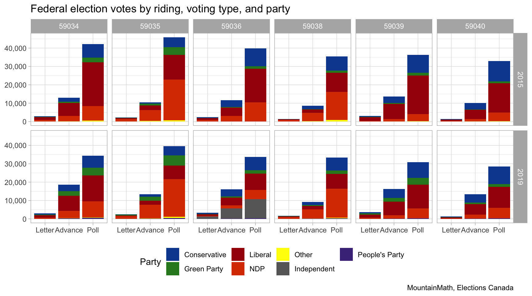
There are few people voting by letter in each riding, but the number of people voting in advance polls is quite substantial. If we are mapping polling district level data, we are only counting the votes of the people that voted in person at the polls. If people living in a polling district voting in advance polls vote substantially different from people voting on election day, then polling district level map won’t accurately reflect the voting pattern living in the polling district.
That’s a problem if we want to do serious analysis with the data, but for today we are mostly interested in how to apply TongFen to this data. For now we will just take a quick peak at differences in shares of votes by voting method, this gives some indication how the different campaigns have structures their get-out-the-vote initiatives.
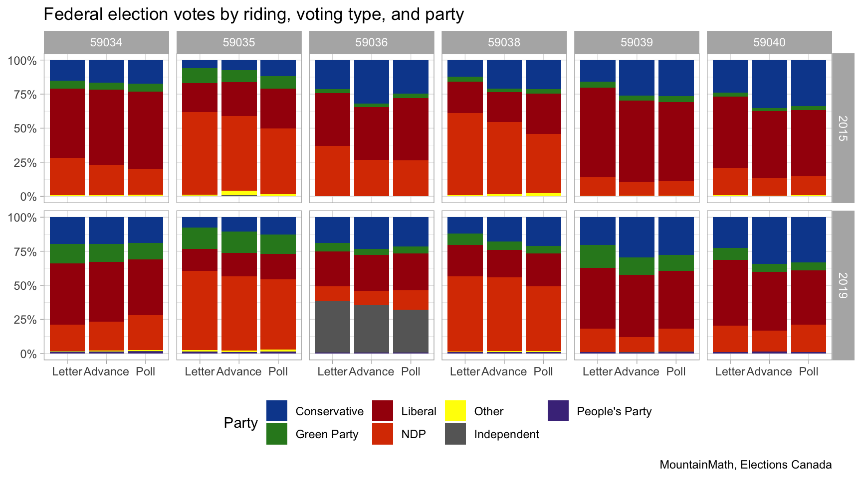
With that done, it’s time to dive into TongFen. The main step is to generate the correspondence estimates. Visual inspection shows that polling districts generally also follow block outlines and are in size not dissimilar from dissemination ares. So we will use the same tolerance of 30m for this.
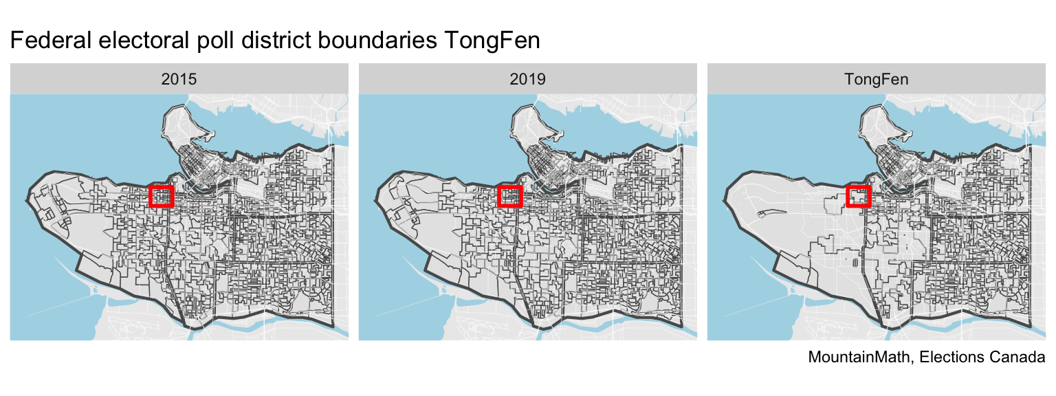
The east side looks fairly intact after TongFen. Areas on the west side have changes considerably, which translates into large agglomerations of poll areas through TongFen. This is emphasized by polling areas on the west side being larger, due to lower population density but also large green areas like the Pacific Spirit Park. If one was interested in a more detailed analysis it might pay of to first cut out large unpopulated areas and thus ignoring boundary changes that do not result in people getting moved to a different polling district.
To better understand the mechanics we focus in on the red square in Kitsilano.
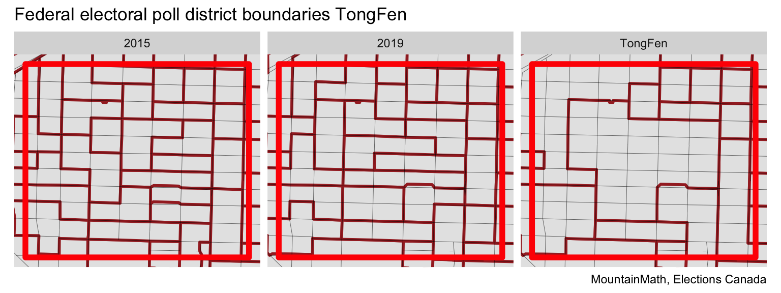
We observe many boundary changes in the centre of the area, as well as the left side, with smaller changes on the right side of the cutout. Visual inspection confirms that the TongFen works as intended in finding an optimal common tiling.
Time to do some mapping. Now that we have a common tiling based on the 2015 and 2019 polling districts, we can compare the voting data for those elections. At least for the portion of the population that voted at the polls on election day. Here is the percentage point change in votes for each of the larger parties in each area.
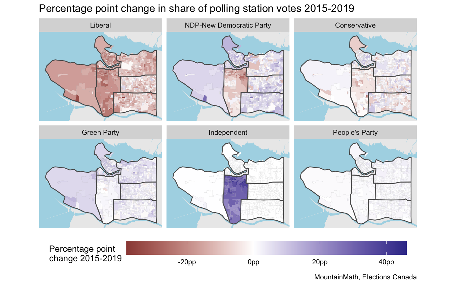
Vancouver Granville stands out, that’s where Jody Wilson-Raybould ran as a Liberal in 2015 and as Independent in 2019. On the east side, where we have retained a fairly granular geographic breakdown, we notice interesting patterns of diverging vote movement.
We can repeat a similar process for the people that voted in advance polls by first aggregating polling districts that had a common advance poll station, and then using TongFen to bring these advance polling districts onto a common geography.
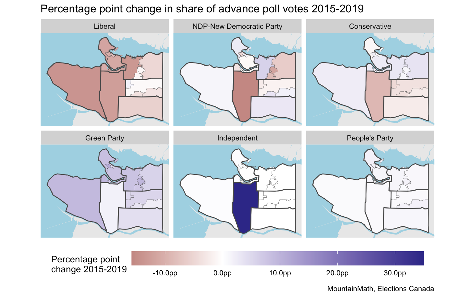
For Vancouver Granville the advance poll data confirms observations from the election day poll seen above that show that the vote swing away from Liberal was in line with many of the adjacent areas, and NDP as well as conservatives also significantly contributed to Jody Wilson-Raybould’s vote total. But that’s something we can already read off from the riding level summaries at the top of this section and does not require TongFen.
Bottom line, while there is some geographic variation visible, most of the interesting story about voter migration happens at the riding level. One interesting sub-riding level story might be in Vancouver East, where advance polling data shows an increase in NDP votes on the western side and a decrease on the east, while election day polling district data shows the reverse. A mirrored pattern can be observed in the Liberal vote change, partially masked by an overall decline in their vote share.
Upshot
Our new estimate_tongfen_correspondence opens the door to universal TongFen, enabling quick and easy estimation of correspondence data for different geographic breakdowns. It find the least common denominator geography, given a specified tolerance, and enables us to make the data geographically comparable.
This is only useful if the different geographic breakdowns are sufficiently congruent, if not we will have to resort to the traditional tongfen_estimate and make due with estimates instead of exact counts. A logical next step would be to round up the functionality of tongfen_estimate by adding an easy way to do sensitivity analysis. But that will require some thinking and will have to wait for another day.
As usual, the code for this post is available on GitHub for anyone to reproduce or adapt for their own TongFen project.
Reproducibility receipt
## [1] "2020-05-20 22:00:00 PDT"## Local: master /Users/jens/Google Drive/R/mountaindoodles
## Remote: master @ origin (https://github.com/mountainMath/doodles.git)
## Head: [6983afd] 2020-05-14: refine text and add health region breakdown graphs## R version 4.0.0 (2020-04-24)
## Platform: x86_64-apple-darwin17.0 (64-bit)
## Running under: macOS Catalina 10.15.4
##
## Matrix products: default
## BLAS: /Library/Frameworks/R.framework/Versions/4.0/Resources/lib/libRblas.dylib
## LAPACK: /Library/Frameworks/R.framework/Versions/4.0/Resources/lib/libRlapack.dylib
##
## locale:
## [1] en_CA.UTF-8/en_CA.UTF-8/en_CA.UTF-8/C/en_CA.UTF-8/en_CA.UTF-8
##
## attached base packages:
## [1] stats graphics grDevices utils datasets methods base
##
## other attached packages:
## [1] mountainmathHelpers_0.1.1 sf_0.9-3
## [3] tongfen_0.1.1 cancensus_0.2.2
## [5] forcats_0.5.0 stringr_1.4.0
## [7] dplyr_0.8.99.9003 purrr_0.3.4
## [9] readr_1.3.1 tidyr_1.0.2
## [11] tibble_3.0.1 ggplot2_3.3.0
## [13] tidyverse_1.3.0
##
## loaded via a namespace (and not attached):
## [1] nlme_3.1-147 fs_1.4.1 lubridate_1.7.8 httr_1.4.1
## [5] rmapzen_0.4.2 tools_4.0.0 backports_1.1.6 R6_2.4.1
## [9] KernSmooth_2.23-16 rgeos_0.5-2 DBI_1.1.0 lazyeval_0.2.2
## [13] colorspace_1.4-1 withr_2.2.0 sp_1.4-1 tidyselect_1.1.0
## [17] git2r_0.26.1 curl_4.3 compiler_4.0.0 cli_2.0.2
## [21] rvest_0.3.5 geojsonsf_1.3.3 xml2_1.3.2 labeling_0.3
## [25] bookdown_0.18 scales_1.1.1 rmapshaper_0.4.4 classInt_0.4-3
## [29] digest_0.6.25 foreign_0.8-78 rmarkdown_2.1 pkgconfig_2.0.3
## [33] htmltools_0.4.0 dbplyr_1.4.3 jsonvalidate_1.1.0 rlang_0.4.6
## [37] readxl_1.3.1 rstudioapi_0.11 httpcode_0.3.0 generics_0.0.2
## [41] farver_2.0.3 jsonlite_1.6.1 magrittr_1.5 Rcpp_1.0.4.6
## [45] munsell_0.5.0 fansi_0.4.1 lifecycle_0.2.0 stringi_1.4.6
## [49] yaml_2.2.1 jqr_1.1.0 grid_4.0.0 maptools_0.9-9
## [53] crayon_1.3.4 geojsonio_0.9.2 lattice_0.20-41 haven_2.2.0
## [57] geojson_0.3.2 hms_0.5.3 knitr_1.28 pillar_1.4.4
## [61] geojsonlint_0.4.0 codetools_0.2-16 crul_0.9.0 reprex_0.3.0
## [65] glue_1.4.1 evaluate_0.14 blogdown_0.18 V8_3.0.2
## [69] modelr_0.1.6 vctrs_0.3.0 cellranger_1.1.0 gtable_0.3.0
## [73] assertthat_0.2.1 xfun_0.13 broom_0.5.6 e1071_1.7-3
## [77] class_7.3-16 ggspatial_1.1.1 units_0.6-6 ellipsis_0.3.1Reuse
Citation
@misc{toward-universal-tongfen-change-in-polling-district-voting-patterns.2020,
  author = {{von Bergmann}, Jens},
  title = {Toward Universal {TongFen:} {Change} in Polling District
    Voting Patterns},
  date = {2020-05-20},
  url = {https://doodles.mountainmath.ca/posts/2020-05-20-toward-universal-tongfen-change-in-polling-district-voting-patterns/},
  langid = {en}
}