Canadian 1996 census data is now avaiable on CensusMapper for anyone to make maps, for API access and via the {cancensus} R package. Yay!
The geographic data is not freely available from Statistics Canada, but can be custom ordered (via a small processing fee). Now the data is freely available on CensusMapper. The geographic data is slightly processed, we clipped out water areas and geographies from CSD upward are slightly simplified for better mapping performance as usual on CensusMapper. I threw the raw data from StatCan into an S3 bucket for download in case anyone is interested in the original data and does not want to pay the processing free.
A little history
We have been slowly expanding the data available via CensusMapper. CensusMapper started out with 2011 Census and NHS data, a flexible tool to map census data that we opened up to the general public for anyone to make their own maps.
While waiting for the 2016 census we added 2006 census data to CensusMapper, our main focus was still on mapping.
As 2016 census data started to trickle in we updated CensusMapper with the new data and build a common tiling of 2006 and 2011 census data to directly compare the two censuses on fine geographies.
It quickly became clear that just mapping the data was inadequate, maps aren’t analysis. To deal with the increasing mess of our analysis pipeline we expanded CensusMapper to serve data via APIs and built the {cancensus} R package as a standardized starting point for reproducible data analysis. And we started to publish the code for our analysis on GitHub and soon after moved our blog over to blogdown for tighter integration of code and version control of our posts, with a strong emphasis on transparency, reproducibility and adaptability of our analysis.
As we shifted away from mapping and toward data analysis, timelines became increasingly important. We added data for the 2001 census and started work on tongfen, a package that automates the process of making census data longitudinally comparable on fine geographies.
Through our work we were able to add custom tabulations to CensusMapper and make them publicly available for mapping or via the API. We also added annual census tract based T1FF taxfiler data all the way back to 2000.
The 2000 T1FF taxfiler data comes on 1996 census geographies, which gave us the final motivation to add the 1996 census. We have been eyeballing this for a while, but one holdup has been that we have not been able to find the geographic data for the 1996 census on a clean open data licence. The data is available through various portals, but not in a way that we can freely distribute it through CensusMapper with just the regular Statistics Canada Open Licence that underlies all the other data on CensusMapper. And now 1996 data is also available on CensusMapper, complete with metadata.
How to use 1996 data
The 1996 data follows a different geographical hierarchy pattern than the 2001-2016 censuses. Instead of Dissemination Areas (DA) it has Enumeration Areas (EA) as the finest geography with all census variables, and it does not have Dissemination Block (DB) data.
That requires a slight change to the {cancensus} package to allow querying of EA level data, which we will get ready from CRAN in the coming weeks. To simplify things, the CensusMapper API server will translate requests for 1996 DA level data (which does not exists) to 1996 EA level data, even though these geographies are quite different and DA/EA level {tongfen} will produce results that are essentially equivalent to CT level {tongfen}.
Moreover, the dataset identifier for the 1996 data (CA1996) does not follow the pattern of the 2001-2016 data where we only used the last two digits of the year (CA01, CA06, CA11, CA16). When we started CensusMapper, we did not anticipate going back that far that we want full years in the labelling. In retrospect that’s a mistake, and we will likely migrate to more consistent naming (without breaking backward compatibility).
Keeping this in mind, we pick a simple census variable, the share of dwelling units in need of major repair, and set up the data import. For each census year we pick out the variables we need via that CensusMapper graphical API interface, specify the geographic region of interest (City of Vancouver in this case), and string the data for the 1996 through 2016 censuses together.
variables <- list(
  CA1996=c(repairs="v_CA1996_1687", all= "v_CA1996_1678"),
  CA01 = c(repairs="v_CA01_104", all= "v_CA01_96"),
  CA06 = c(repairs="v_CA06_108", all= "v_CA06_105"),
  CA11 = c(repairs="v_CA11N_2232", all= "v_CA11N_2230"),
  CA16 = c(repairs="v_CA16_4872", all= "v_CA16_4870")
)
regions <- list(CSD="5915022")

get_dwelling_condition <- function(regions,variables,level="Regions",geo_format=NA) {
  names(variables) %>% lapply(function(dataset){
    year=str_extract(dataset,"\\d+")
    if (nchar(year)==2) year=paste0("20",year)
    get_census(dataset,regions=regions, vectors=variables[[dataset]],
               level=level, geo_format=geo_format) %>%
      mutate(Year=year)
  }) %>%
    bind_rows() %>%
    mutate(share=repairs/all) %>%
    mutate(share_d=pretty_cut(share,c(-Inf,0.05,0.1,0.15,0.2,0.3,0.4,Inf),
                              format = scales::percent,ordered_result=TRUE))
}
First we query the city-wide data.
data <- get_dwelling_condition(regions,variables)
colours <- setNames(viridis::viridis(length(levels(data$share_d))),levels(data$share_d))

ggplot(data,aes(x=as.character(Year),y=share)) +
  geom_bar(stat="identity",fill="brown") +
  scale_y_continuous(labels=scales::percent) +
  labs(title="City of Vancouver homes in need of major repairs",
       y="Share of homes in need of major repairs",
       x=NULL,
       caption="MountainMath, StatCan Census 1996-2016")
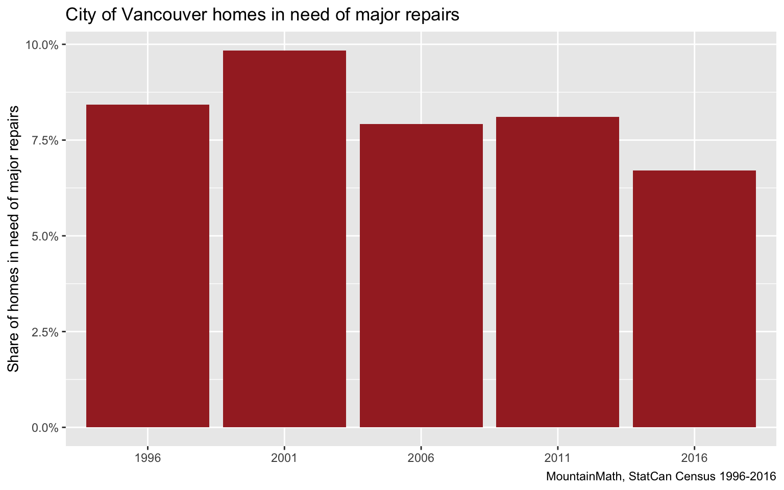
The share of dwellings in need of major repairs reached a peak in 2001 and slowly decreased after, possibly an effect of the leaky condo crisis. This kind of data is best checked via a cross tabulation.

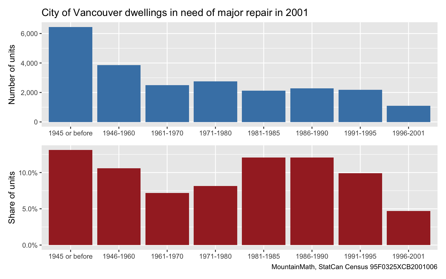
We would expect the share of buildings in need of major repairs to increase with building age, but looking at the data we see that buildings between 1981 and 1995 (and maybe even up to 2001) show a heightened share of buildings in need of major repairs. Using a crude estimate of maybe half of those units been 1951 and 2001 being due to leaky condos, they make an overall contribution of 1.1 percentage points to the share of dwellings in need of major repairs. Which explains much of the jump.
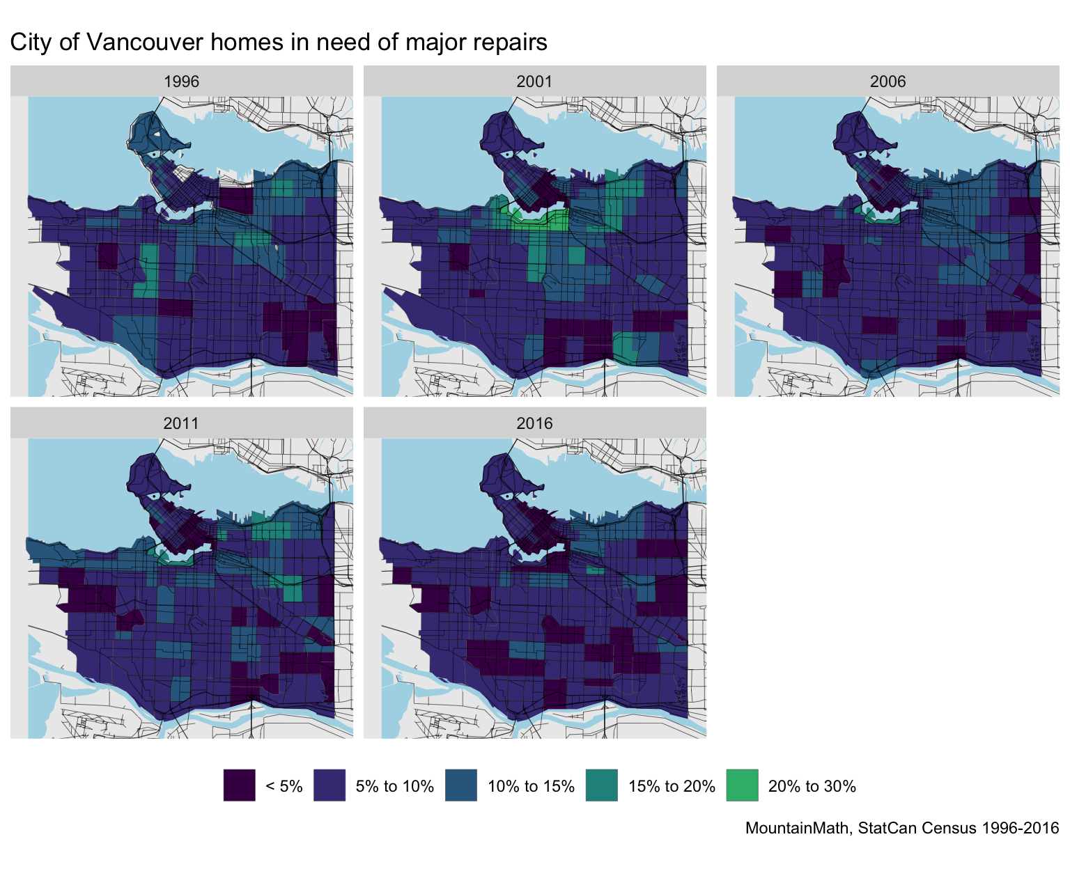
Mapping the share of homes in need of major repairs might help us understand this better. We start out with Census Tract level.
ggplot(get_dwelling_condition(regions,variables,level="CT",geo_format='sf')) +
  geom_sf(aes(fill=share_d),size=0.1) +
  scale_fill_manual(values=colours,na.value="darkgrey") +
  map_theme +
  labs(title="City of Vancouver homes in need of major repairs")
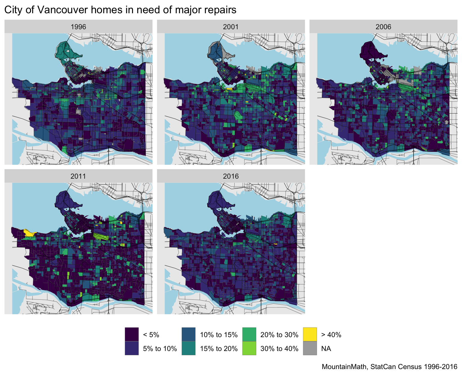
There is clear geographic variability, it might be worthwhile to zoom in to DA/EA level data.
ggplot(get_dwelling_condition(regions,variables,"DA",'sf')) +
  geom_sf(aes(fill=share_d),size=0.1) +
  scale_fill_manual(values=colours,na.value="darkgrey") +
  map_theme +
  labs(title="City of Vancouver homes in need of major repairs")
We notice quite a bit of volatility in the data, both geographically and temporally. We will leave it to another post to explore the relationships of dwellings in disrepair with other variables. People that have been following the leaky condo and other developments with major deficiencies more closely might be able to make sense of these patterns just by looking at the maps.
Upshot
Timelines matter a lot for analysis, and it’s great to have one more census conveniently available for mapping and API access. As usual, the full code for this post is available on GitHub.
Reuse
Citation
@misc{canadian-1996-census.2020,
  author = {{von Bergmann}, Jens},
  title = {Canadian 1996 {Census}},
  date = {2020-07-06},
  url = {https://doodles.mountainmath.ca/posts/2020-07-06-canadian-1996-census/},
  langid = {en}
}